Copying "Introduction to Statistical Analysis" in Python Vol. 9 - Chapter 4 "First Statistical Tests" ② Testing the Difference Between Two Population Means

Chapter 4 "First Statistical Tests"

Book Author: Dr. Sadao Ishimura

This article covers the "Introduction to Statistical Analysis" book, Chapter 4 "First Statistical Tests", Python coding activity.

This is a coding series where I calmly convert the book's figures, tables, and calculations into Python.
In this article, among the statistical test themes in Chapter 4, I will tackle testing the difference between two population means and testing the difference between two paired population means.
I will also continue to utilize ChatGPT!

Now, let's open the book and set off on a journey of statistical analysis 🚀

Introduction

This blog series introduces the "joy of statistical analysis" gained through Python coding of the book "Introduction to Statistical Analysis" (Tokyo Tosho, referred to as the "textbook").

The book introduction and citation notation are posted in the linked article.

Chapter 4 First Statistical Tests

This article covers the following sections of Chapter 4.

The data used in the article is cited directly from the data published in the textbook.
For items with a small amount of data, I register the data in the code, and for items with a large amount of data, I create a CSV file and load the data.

I will import the libraries used in Chapter 4.

### インポート

# 数値計算
import math                                                # python標準ライブラリ
import numpy as np
import pandas as pd

# 統計
import scipy.stats as stats
import pingouin as pg
from statsmodels.stats.proportion import proportions_ztest # 母比率のz検定
from statsmodels.stats.weightstats import ttest_ind        # 2標本のt検定

# 描画
import matplotlib.pyplot as plt
import seaborn as sns
plt.rcParams['font.family'] = 'Meiryo'

Introduction

Here is an introduction drafted together with ChatGPT!

"Which store had better customer service, Store A or Store B?" "Is the new version of this product really easier to use than the old version?"
In our daily lives, we often compare two things to make a judgment.

Statistics also has tools for "comparing and judging."
That is the theme of this time, tests of difference.
The point this time is collecting data (=samples) from two groups and seeing if there is a difference.

"Is there a difference?" "Is it just a coincidence?"
The role of the test of difference is to firmly answer such questions based on two samples.

Let's continue to work hard on "statistical tests."
First, please enjoy the "gentle intro" to "tests of difference" by ChatGPT.

In the previous article, we learned about testing for a "single population."
This time, we will step up and tackle the scenario of "comparing two populations."While focusing on the "differences" that become visible through comparison, let's take a gentle look at the following four tests.

🍰 A gentle introduction to each test

🔸 Test for the difference between two population means
→ This is a test to investigate whether there is a difference in the "mean" of two populations, such as "Is there a difference in average annual income between Company A and Company B?"whether there is a difference in the "mean" of two populations is the goal of this test.

🔸 Test for the difference between two paired population means
→ This investigates the difference in means when "the same subject is measured twice," such as "Did the same person's weight change before and after a diet?""the same subject measured twice" is what we investigate.
→ This is used when the comparison partner is not a "different person" but rather "the same person's before and after."

✨ Closing the intro
Every test is a tool for determining, "Is the difference real? Or is it just a coincidence?"
Let's take the first step together toward drawing reliable comparisons from data.

Section 4.5 Test for the difference between two population means

The difference between the population means of two normal populations will be handled.

[Hypothesis]
We set the hypothesis for the difference in population means $${\mu_1 - \mu_2}$$ that we wish to overturn as follows.

The hypothesis we wish to support, the alternative hypothesis, is set as one of the following three patterns.

◆ ◆ ◆

■ Test for the difference between two population means (assuming equal variance): Formula for test statistic p.162
I will borrow the formula for the test statistic in the test for the difference between two population means (population variance unknown, assuming equal variance) from the text.

Test statistic for the difference between two population means $${\mu_1 - \mu_2}$$ using two samples $${\{x_{11}, x_{12}, \ldots, x_{1N_1}\}}$$ and $${\{x_{21}, x_{22}, \ldots, x_{2N_2}\}}$$

follows a $${t}$$ distribution with degrees of freedom $${N_1+N_2-2}$$.
If we replace the subscripts $${_{1, 2}}$$ indicating group 1 and group 2 with $${_i}$$, then $${\bar{x_i}}$$ is the sample mean and $${N_i}$$ is the sample size.
$${s^2}$$ is called the "pooled variance" and is calculated using the following formula using the sample variance $${s_i^2}$$ of each group.

Define the "test function for the difference between two population means" according to the formula.
Use scipy.stats for probability calculations.

### ２つの正規母集団の母平均の差の検定関数 p.162

# ２つの正規母集団の母平均の差のt検定統計量の算出関数
def t_stat_pop_mean_diff(x_list1, x_list2, mu01=0, mu02=0):
    # 各グループの標本サイズ
    N1, N2 = len(x_list1), len(x_list2)
    # 各グループの標本平均
    x_bar1, x_bar2 = sum(x_list1) / N1, sum(x_list2) / N2
    # 各グループの標本分散
    s21 = sum([(x1 - x_bar1)**2 for x1 in x_list1]) / (N1 - 1)
    s22 = sum([(x2 - x_bar2)**2 for x2 in x_list2]) / (N2 - 1)
    # s²
    s2 = ((N1 - 1)*s21 + (N2 - 1)*s22) / (N1 + N2 - 2)
    # 戻り値: t検定統計量
    return ((x_bar1 - x_bar2) - (mu01 - mu02)) / math.sqrt((1/N1 + 1/N2)*s2)

# ２つの正規母集団の母平均のt検定関数 ※確率計算はscipy.stats利用
def pop_mean_diff_ttest(
        x_list1, x_list2, mu01=0, mu02=0, alpha=0.05, alternative='two-sided'):
    # 各グループの標本サイズ
    N1, N2 = len(x_list1), len(x_list2)
    # t検定統計量の算出
    t_val = t_stat_pop_mean_diff(x_list1, x_list2, mu01, mu02)
    # 自由度(N1+N2-2)のt分布の設定
    t_dist = stats.t(df=N1 + N2 - 2)
    # 棄却限界値c_valとp値p_valの算出
    match alternative:
        case 'two-sided':
            c_val = t_dist.ppf(q=1 - alpha/2)
            c_val = -c_val, c_val
            p_val = t_dist.sf(x=abs(t_val)) * 2
        case 'less':
            c_val = t_dist.ppf(q=alpha)
            p_val = t_dist.cdf(x=t_val)
        case 'greater':
            c_val = t_dist.ppf(q=1 - alpha)
            p_val = t_dist.sf(x=t_val)
    return {'t_value': t_val, 'c_value': c_val, 'alpha': alpha, 'p_value': p_val}

For test data $${[1, 2, 3]}$$ and $${[1.5, 1.8, 2.0]}$$, perform a test of population means with the null hypothesis $${H_0}$$ "difference in population means $${\mu_1 > \mu_2}$$," a significance level of 5% ($${\alpha=0.05}$$), and a two-tailed test.

# テスト
x_list1, x_list2 = [1, 2, 3], [1.5, 1.8, 2.0]
pop_mean_diff_ttest(x_list1, x_list2, alternative='greater')

【Execution Result】
"Not significant at the 5% significance level, so the null hypothesis cannot be rejected."

Briefly explain the output content.

• t_value: Realized value of the test statistic $${T}$$

• c_value: Critical value
  Threshold for the test statistic $${T}$$ at which the null hypothesis can be rejected
  When the realized value of $${T}$$ is outside the critical value, the null hypothesis can be rejected

• alpha: Significance level $${\alpha}$$

• p_value: $${p}$$ value
  Probability that the test statistic becomes the realized value under the null hypothesis
  When the $${p}$$ value is less than or equal to the significance level, the null hypothesis can be rejected

Verify the calculation using scipy.stats.

### scipy.statsで答え合わせ
stats.ttest_ind(x_list1, x_list2, equal_var=True, alternative='greater')

【Execution Result】
Test statistic and $${p}$$ value.
The verification results match.

◆ ◆ ◆

■ Test of the difference between two population means (two-tailed test) Example p.164
Example on p.164: Investigate whether there is a difference in the body length of char inhabiting the "Tone River system" and the "Shinano River system" using a test for the difference between two population means.

The hypotheses are as follows:
・Null hypothesis $${H_0}$$ "Difference in population means $${\mu_1=\mu_2}$$"
・Alternative hypothesis $${H_1}$$ "Difference in population means $${\mu_1 \neq \mu_2}$$"
　⇒Two-tailed test: Interested in the presence or absence of a difference regardless of the magnitude of the difference

① Perform the test using a custom function
First, set the two datasets.

### ２つの母平均の差の検定（両側検定） イワナの体長 p.164

# データ
tone = [165, 130, 182, 178, 194, 206, 160, 122, 212, 165, 247, 195]
shinano = [180, 180, 235, 270, 240, 285, 164, 152]

Next, perform the test for the difference between two population means with a significance level of $${5\%}$$ and a two-tailed test.

# 関数利用
result = pop_mean_diff_ttest(tone, shinano)
result

【Execution Result】
The test statistic $${T=-1.765}$$ is greater than the critical value (lower threshold) $${-2.101}$$ (according to the text, it does not fall into the rejection region), so the null hypothesis cannot be rejected at the $${5\%}$$ significance level.

In other words, itcannot be said that there is a differencein the body length of char between the two rivers.

② Visualization of the test
Let's visualize the $${t}$$ distribution to see how it cannot be rejected.

### 図示 p.166

## 設定と準備
# 統計関連の値
N1, N2 = len(tone), len(shinano)  # 標本サイズ
alpha = result['alpha']           # 有意水準
lower, upper = result['c_value']  # 棄却限界値
t_val = result['t_value']         # 検定統計量
t_dist = stats.t(df=N1 + N2 - 2)  # t分布
# グラフ描画用設定
color = 'tab:blue'                            # 基本の色
x_min, x_max = -5, 5                          # x軸の最小値、最大値
x_val = np.linspace(x_min, x_max, 1001)       # 確率密度関数用のx軸の値
x_val_lower = np.linspace(x_min, lower, 101)  # 下側棄却域用のx軸の値
x_val_upper = np.linspace(upper, x_max, 101)  # 上側棄却域用のx軸の値

## 描画処理
# 描画領域の設定
plt.figure(figsize=(7, 3))
# t分布の確率密度関数の描画
plt.plot(x_val, t_dist.pdf(x_val), color=color,
         label=f'自由度({N1}+{N2}-2)の$t$分布')
# 下側棄却域の塗りつぶし
plt.fill_between(x_val_lower, 0, t_dist.pdf(x_val_lower),
                 color=color, alpha=0.3, label=f'有意水準{alpha}の棄却域')
# 上側棄却域の塗りつぶし
plt.fill_between(x_val_upper, 0, t_dist.pdf(x_val_upper),
                 color=color, alpha=0.3)
# 検定統計量の垂直線の描画
plt.axvline(t_val, color='tab:red', ls='--', label=f'検定統計量={t_val:.3f}')
# 修飾
plt.xticks([lower, 0, upper])
plt.legend();

[Execution Results]

The bell-shaped curve is the probability density function of the t-distribution with degrees of freedom $${N_1+N_2-2=18}$$ .
The blue regions at both ends are the rejection regions at the significance level of $${5\%}$$ .
Since it is a two-sided test, there is a $${2.5\%}$$ rejection region at each end.
The red dotted line is the test statistic $${T}$$ .

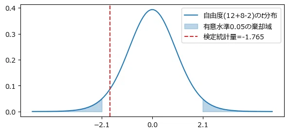
Since $${T}$$ does not fall into either rejection region, the null hypothesis cannot be rejected.

③ Executing the test with Python libraries
Usually, it is best to utilize well-established libraries.
Here, we will use scipy.stats, pingouin, and statsmodels.
All of them take the two sample datasets and the assumption of equal variance as arguments.

🖲️scipy.stats

# scipy.stats利用
stats.ttest_ind(tone, shinano, equal_var=True)

[Execution Results]
We obtained the test statistic $${T}$$, the $${p}$$-value, and the degrees of freedom of the t-distribution.

🖲️pingouin

# pingouin利用
pg.ttest(x=tone, y=shinano, correction=False)  # correction=True: ウェルチのt検定

[Execution Results]
The main outputs are: T: test statistic $${T}$$, p-val: $${p}$$-value, CI95%: 95% confidence interval, and effect size (Cohen's d).

💡 Inserting Tips
Effect size is a reference value for the "magnitude of the difference."
The test statistic and $${p}$$-value in a difference test tell you about the "presence or absence of a difference."
It seems that effect size is used as a reference for the "magnitude of the difference."
The following web article is helpful.

🖲️statsmodels

# statsmodels利用
ttest_ind(tone, shinano, usevar='pooled')

[Execution Results]
We obtained the test statistic $${T}$$, the $${p}$$-value, and the degrees of freedom of the t-distribution.

◆ ◆ ◆

■ Test for the difference between two population means (one-sided test) Example p.168
Using the example on p.164, we will examine whether charr living in the "Shinano River system" (a cold-water system) are larger in body length than those in the "Tone River system" using a test for the difference between two population means.

The hypotheses are as follows:
・Null hypothesis $${H_0}$$: "Difference in population means $${{\mu_1=\mu_2}}$$"
・Alternative hypothesis $${H_1}$$: "Difference in population means $${{\mu_1 < \mu_2}}$$"
　⇒One-sided test (less): Interested in whether group 2 is larger

① Executing the test with a custom function
First, we set up the two datasets.

### ２つの母平均の差の検定（両側検定） イワナの体長 p.168

# データ
tone = [165, 130, 182, 178, 194, 206, 160, 122, 212, 165, 247, 195]
shinano = [180, 180, 235, 270, 240, 285, 164, 152]

Next, we execute the test for the difference between two population means with a significance level of $${5\%}$$ and a one-sided test (less).

# 関数利用
result = pop_mean_diff_ttest(tone, shinano, alternative='less')
result

[Execution Results]
The test statistic $${T=-1.765}$$ is smaller than the rejection limit (lower threshold) of $${-1.734}$$ (according to the text, it falls into the rejection region), so the null hypothesis is rejected at the $${5\%}$$ significance level.

In other words,it can be said that the charr in the Shinano River system have a larger body length.

② Visualization of the test
Let's visualize the t-distribution to see how it is rejected.

### 図示 p.166

## 設定と準備
# 統計関連の値
N1, N2 = len(tone), len(shinano)  # 標本サイズ
alpha = result['alpha']           # 有意水準
lower = result['c_value']         # 棄却限界値
t_val = result['t_value']         # 検定統計量
t_dist = stats.t(df=N1 + N2 - 2)  # t分布
# グラフ描画用設定
color = 'tab:blue'                            # 基本の色
x_min, x_max = -5, 5                          # x軸の最小値、最大値
x_val = np.linspace(x_min, x_max, 1001)       # 確率密度関数用のx軸の値
x_val_lower = np.linspace(x_min, lower, 101)  # 下側棄却域用のx軸の値

## 描画処理
# 描画領域の設定
plt.figure(figsize=(7, 3))
# t分布の確率密度関数の描画
plt.plot(x_val, t_dist.pdf(x_val), color=color,
         label=f'自由度({N1}+{N2}-2)の$t$分布')
# 下側棄却域の塗りつぶし
plt.fill_between(x_val_lower, 0, t_dist.pdf(x_val_lower),
                 color=color, alpha=0.3, label=f'有意水準{alpha}の棄却域')
# 検定統計量の垂直線の描画
plt.axvline(t_val, color='tab:red', ls='--', label=f'検定統計量={t_val:.3f}')
# 修飾
plt.xticks([lower, 0])
plt.legend();

[Execution Results]

The bell-shaped curve is the probability density function of the t-distribution with degrees of freedom $${N_1+N_2-2=18}$$.
The blue area on the left (lower side) is the rejection region at a significance level of $${5\%}$$.
The red dotted line is the test statistic $${T}$$.

Since $${T}$$ falls within the rejection region, the null hypothesis is rejected.

③ Executing the test with Python libraries
We will use scipy.stats, pingouin, and statsmodels.
In all cases, the arguments passed are the two sample datasets, the assumption of equal variance, and the one-sided test (less).

🖲️scipy.stats

# scipy.stats利用
stats.ttest_ind(tone, shinano, equal_var=True, alternative='less')

【Execution Results】
We obtained the test statistic $${T}$$, the $${p}$$-value, and the degrees of freedom for the t-distribution.

🖲️pingouin

# pingouin利用
pg.ttest(x=tone, y=shinano, correction=False, alternative='less')

【Execution Results】
The main outputs are T: test statistic $${T}$$, p-val: $${p}$$-value, and CI95%: 95% confidence interval.

🖲️statsmodels

# statsmodels利用
ttest_ind(tone, shinano, usevar='pooled', alternative='smaller')

【Execution Results】
We obtained the test statistic $${T}$$, the $${p}$$-value, and the degrees of freedom for the t-distribution.

■ Test for the difference between two population means (when equal variance is not assumed): Formula for the test statistic p.171
From here on, we will deal with cases where "the population variances of the two groups are different / no assumption is made that the population variances are equal."

We borrow the formula for the test statistic in the test for the difference between two population means (population variance unknown, equal variance not assumed), commonly known as Welch's test, from the text.

Test statistic for the difference between two population means $${\mu_1 - \mu_2}$$ using two samples $${{x_{11}, x_{12}, \ldots, x_{1N_1}}}$$ and $${{x_{21}, x_{22}, \ldots, x_{2N_2}}}$$

follows a t-distribution with degrees of freedom $${m}$$.
If we replace the subscripts $${_{1, 2}}$$ indicating group 1 and group 2 with $${_i}$$, then $${{\bar{x}_i}}$$ is the sample mean, $${s^2}$$ is the sample variance, and $${N_i}$$ is the sample size.

The degrees of freedom $${m}$$ are approximated by the following formula.
When $${m}$$ is not an integer, the nearest integer value is taken as $${m}$$.

We define a "Welch's test function" according to the formula.
We use scipy.stats for probability calculations.
Note that the degrees of freedom $${m}$$ for this function will be kept as a decimal value rather than an integer.

### ２つの正規母集団の母平均の差の検定関数 p.162

# ２つの正規母集団の母平均の差のウェルチのt検定統計量の算出関数
def t_stat_welch_pop_mean_diff(list1, list2, mu01=0, mu02=0):
    # 各グループの標本サイズ
    N1, N2 = len(list1), len(list2)
    # 各グループの標本平均
    x_bar1, x_bar2 = sum(list1) / N1, sum(list2) / N2
    # 各グループの標本分散
    s21 = sum([(x1 - x_bar1)**2 for x1 in list1]) / (N1 - 1)
    s22 = sum([(x2 - x_bar2)**2 for x2 in list2]) / (N2 - 1)
    # 自由度 ※整数値に丸めていない（scipy.stats等と同様にfloat型の自由度にする）
    m = (s21/N1 + s22/N2)**2 / \
        (s21**2/(N1**2 * (N1 - 1)) + s22**2/(N2**2 * (N2 - 1)))
    # 戻り値: ウェルチのt検定統計量, 自由度m
    return ((x_bar1 - x_bar2) - (mu01 - mu02)) / (s21/N1 + s22/N2)**(1/2), m

# ２つの正規母集団の母平均のウェルチのt検定関数 ※確率計算はscipy.stats利用
def pop_mean_diff_welch_ttest(
        list1, list2, mu01=0, mu02=0, alpha=0.05, alternative='two-sided'):
    # t検定統計量と自由度の算出
    t_val, m = t_stat_welch_pop_mean_diff(list1, list2, mu01, mu02)
    # 自由度(m)のt分布の設定
    t_dist = stats.t(df=m)
    # 棄却限界値c_valとp値p_valの算出
    match alternative:
        case 'two-sided':
            c_val = t_dist.ppf(q=1 - alpha/2)
            c_val = -c_val, c_val
            p_val = t_dist.sf(x=abs(t_val)) * 2
        case 'less':
            c_val = t_dist.ppf(q=alpha)
            p_val = t_dist.cdf(x=t_val)
        case 'greater':
            c_val = t_dist.ppf(q=1 - alpha)
            p_val = t_dist.sf(x=t_val)
    return {'t_value': t_val, 'c_value': c_val, 'alpha': alpha,
            'p_value': p_val, 'df': m}

For the test data $${[1, 2, 3]}$$ and $${[1.5, 1.8, 2.0]}$$, we perform a test for the population means with the null hypothesis $${H_0}$$ "difference in population means $${{\mu_1 > \mu_2}}$$," a significance level of 5% ($${{\alpha=0.05}}$$ ), and a two-sided test.

# テスト
list1, list2 = [1, 2, 3], [1.5, 1.8, 2.0]
pop_mean_diff_welch_ttest(list1, list2, alternative='greater')

[Execution Result]
"It cannot be said to be significant at the 5% significance level, and the null hypothesis cannot be rejected."

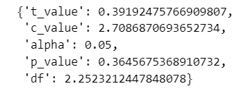
I will briefly explain the output content.

• t_value: The realized value of the test statistic $${T}$$

• c_value: Critical value
  The threshold for the test statistic $${T}$$ at which the null hypothesis can be rejected
  When the realized value of $${T}$$ is outside the critical value, the null hypothesis can be rejected

• alpha: Significance level $${\alpha}$$

• p_value: $${p}$$ value
  The probability that the test statistic becomes the realized value under the null hypothesis
  When the $${p}$$ value is less than or equal to the significance level, the null hypothesis can be rejected

• df: Degrees of freedom

I will verify the calculation using scipy.stats.

### scipy.statsで答え合わせ ※equal_var=Falseでウェルチの検定になる
stats.ttest_ind(list1, list2, equal_var=False, alternative='greater')

[Execution Result]
These are the test statistic, $${p}$$ value, and degrees of freedom.
The verification results matched.

◆ ◆ ◆

■ Welch's t-test (two-tailed test) Example p.164
We will investigate whether there is a difference in the body length of charr living in the "Tone River system" and the "Shinano River system" from the example on p.172 using Welch's t-test.

The hypotheses are as follows:
・Null hypothesis $${H_0}$$: "Difference in population means $${\mu_1=\mu_2}$$"
・Alternative hypothesis $${H_1}$$: "Difference in population means $${\mu_1 \neq \mu_2}$$"
　⇒ Two-tailed test: Interested in whether there is a difference regardless of the magnitude of the difference

① Execute test with custom function
First, set the two datasets.

### ２つの母平均の差のウェルチの検定（両側検定） イワナの体長 p.172

# データ
tone = [165, 130, 182, 178, 194, 206, 160, 122, 212, 165, 247, 195]
shinano = [180, 180, 235, 270, 240, 285, 164, 152]

Next, perform Welch's t-test with a significance level of $${5\%}$$ and a two-tailed test.

# 関数利用
result = pop_mean_diff_welch_ttest(tone, shinano)
result

[Execution Result]
Since the test statistic $${T=-1.636}$$ is greater than the critical value (lower threshold) $${-2.192}$$ (it does not fall into the rejection region according to the text), the null hypothesis cannot be rejected at the $${5\%}$$ significance level.

In other words, it cannot be said that there is a difference in the body length of charr between the two rivers.

② Visualization of the test
Let's visualize the $${t}$$ distribution to see how it cannot be rejected.

### 図示 p.173

## 設定と準備
# 統計関連の値
N1, N2 = len(tone), len(shinano)  # 標本サイズ
alpha = result['alpha']           # 有意水準
lower, upper = result['c_value']  # 棄却限界値
t_val = result['t_value']         # 検定統計量
df = result['df']                 # 自由度
t_dist = stats.t(df=df)           # t分布
# グラフ描画用設定
color = 'tab:blue'                            # 基本の色
x_min, x_max = -5, 5                          # x軸の最小値、最大値
x_val = np.linspace(x_min, x_max, 1001)       # 確率密度関数用のx軸の値
x_val_lower = np.linspace(x_min, lower, 101)  # 下側棄却域用のx軸の値
x_val_upper = np.linspace(upper, x_max, 101)  # 上側棄却域用のx軸の値

## 描画処理
# 描画領域の設定
plt.figure(figsize=(7, 3))
# t分布の確率密度関数の描画
plt.plot(x_val, t_dist.pdf(x_val), color=color, label=f'自由度{df:.4f}の$t$分布')
# 下側棄却域の塗りつぶし
plt.fill_between(x_val_lower, 0, t_dist.pdf(x_val_lower),
                 color=color, alpha=0.3, label=f'有意水準{alpha}の棄却域')
# 上側棄却域の塗りつぶし
plt.fill_between(x_val_upper, 0, stats.t.pdf(x_val_upper, df=N - 1),
                 color=color, alpha=0.3)
# 検定統計量の垂直線の描画
plt.axvline(t_val, color='tab:red', ls='--', label=f'検定統計量={t_val:.3f}')
# 修飾
plt.xticks([lower, 0, upper])
plt.legend();

[Execution Result]

The bell-shaped curve is the probability density function of the $${t}$$ distribution with $${11.3875}$$ degrees of freedom.
The blue regions at both ends are the rejection regions for the $${5\%}$$ significance level.
Since it is a two-tailed test, there is a $${2.5\%}$$ rejection region at each end.
The red dotted line is the test statistic $${T}$$.

Since $${T}$$ is not in either rejection region, the null hypothesis cannot be rejected.

(3) Executing the test with Python libraries
We will use scipy.stats, pingouin, and statsmodels.
In all cases, we pass the two sample datasets and specify that equal variance is not assumed as arguments.

🖲️scipy.stats

# scipy.stats利用 ※equal_var=False=Trueでウェルチの検定になる
stats.ttest_ind(tone, shinano, equal_var=False)

[Execution Results]
We obtained the test statistic $${T}$$, the $${p}$$-value, and the degrees of freedom for the $${t}$$-distribution.

🖲️pingouin

# pingouin利用 ※correction=Trueでウェルチの検定になる
pg.ttest(x=tone, y=shinano, correction=True)

[Execution Results]
The main outputs are T: test statistic $${T}$$, p-val: $${p}$$-value, and CI95%: 95% confidence interval.

🖲️statsmodels

# statsmodels利用 ※usevar='unequal'でウェルチの検定になる
ttest_ind(tone, shinano, usevar='unequal')

[Execution Results]
We obtained the test statistic $${T}$$, the $${p}$$-value, and the degrees of freedom for the $${t}$$-distribution.

Understanding Check: Testing the Difference Between Two Population Means p.174

This is a test for the difference in population means regarding gender differences in a certain test value.
Assuming equal variance, with a significance level of $${5\%}$$, and using a two-tailed test, we will write the code straightforwardly.

Set the sample data.
sample1 is Group 1: Female, and sample2 is Group 2: Male.

### ２つの母平均の差の検定（両側検定） 総コレステロール値 p.174

# データ
sample1 = [292, 351, 284, 278, 322, 295, 282, 317,
           305, 296, 267, 272, 343, 298, 275]
sample2 = [265, 272, 248, 276, 284, 258, 289, 307,
           284, 273, 301, 268, 293, 284, 318]

Execute the test using a custom function.

# 関数利用
result = pop_mean_diff_ttest(sample1, sample2)
result

[Execution Results]
The null hypothesis is rejected.

Execute the test using scipy.stats.

# scipy.stats利用
stats.ttest_ind(sample1, sample2, equal_var=True)

[Execution Results]

Execute the test using pingouin.

# pingouin利用
pg.ttest(x=sample1, y=sample2, correction=False)

[Execution Results]

Execute the test using statsmodels.

# statsmodels利用
ttest_ind(sample1, sample2, usevar='pooled')

[Execution Results]

Let's visualize the $${t}$$-distribution to see how it can be rejected.

### 図示 p.175

## 設定と準備
# 統計関連の値
N1, N2 = len(sample1), len(sample2)  # 標本サイズ
alpha = result['alpha']              # 有意水準
lower, upper = result['c_value']     # 棄却限界値
t_val = result['t_value']            # 検定統計量
t_dist = stats.t(df=N1 + N2 - 2)     # t分布
# グラフ描画用設定
color = 'tab:blue'                            # 基本の色
x_min, x_max = -5, 5                          # x軸の最小値、最大値
x_val = np.linspace(x_min, x_max, 1001)       # 確率密度関数用のx軸の値
x_val_lower = np.linspace(x_min, lower, 101)  # 下側棄却域用のx軸の値
x_val_upper = np.linspace(upper, x_max, 101)  # 上側棄却域用のx軸の値

## 描画処理
# 描画領域の設定
plt.figure(figsize=(7, 3))
# t分布の確率密度関数の描画
plt.plot(x_val, t_dist.pdf(x_val), color=color,
         label=f'自由度({N1}+{N2}-2)の$t$分布')
# 下側棄却域の塗りつぶし
plt.fill_between(x_val_lower, 0, t_dist.pdf(x_val_lower),
                 color=color, alpha=0.3, label=f'有意水準{alpha}の棄却域')
# 上側棄却域の塗りつぶし
plt.fill_between(x_val_upper, 0, t_dist.pdf(x_val_upper),
                 color=color, alpha=0.3)
# 検定統計量の垂直線の描画
plt.axvline(t_val, color='tab:red', ls='--', label=f'検定統計量={t_val:.3f}')
# 修飾
plt.xticks([lower, 0, upper])
plt.legend();

[Execution Results]

A brief detour: The Brunner-Munzel test

When I was searching online for tests of the difference between two population means, I came across the Brunner-Munzel test.
Since it is a non-parametric test, there is no need to assume that the population follows a normal distribution, nor is there a need to assume equal variance.
Actually, I will be practicing non-parametric tests in Chapter 5, but it does not include the Brunner-Munzel test.
I am presenting it "while it's fresh" (Note: "fresh" is based on my own timing).

📣 Features 📣

• A non-parametric test for two samples that requires neither the assumption of a normal distribution nor the assumption of equal variance

• Detects whether there is a significant difference in the medians of the data

• Null hypothesis: When one value is taken from each group, the probability of obtaining a larger value is equal for both groups

• If the $${p}$$ value is below the significance level, the alternative hypothesis that "there is a difference between the two samples" is supported

I will follow the code from the official scipy website.
This is a two-tailed test.

# Brunner-Munzel検定 scipy.stats公式のコードをなぞってみる
x1 = [1,2,1,1,1,1,1,1,1,1,2,4,1,1]
x2 = [3,3,4,3,1,2,3,1,1,5,4]
w, p_value = stats.brunnermunzel(x1, x2)
w, p_value

[Execution Results]
The statistic and $${p}$$ value were output.
The flow is such that the null hypothesis is rejected at a 5% significance level.

Let's compare it with Welch's test.

# 参考：ウェルチの検定 scipy.stats利用 ※equal_var=False=Trueでウェルチの検定になる
stats.ttest_ind(x1, x2, equal_var=False)

[Execution Results]
The null hypothesis is also rejected here at a 5% significance level.

Looking at the histogram of the data, it does not appear to be a normal distribution.
In the case of this data, it is better to avoid using tests that "assume a normal distribution," such as Welch's test.

# ２つデータのヒストグラム
plt.hist(x1, alpha=0.5, label='$x_1$')
plt.hist(x2, alpha=0.5, label='$x_2$')
plt.legend();

[Execution Results]

If you are interested, please get more information from the following website.

Section 4.6 Testing the difference between two paired population means

■ Introduction
Testing the difference between two paired population means targets the difference in population means of two samples obtained from the "same person" or "same subject".
The two samples have a "paired relationship," and since the difference in population means can be considered as "one population," we use the "one-sample test for population mean" (Section 4.2).

■ Probability distribution followed by the population
The text does not explicitly state the probability distribution followed by the population regarding the test for the difference between two paired population means.
However, since the test for the difference between two paired population means uses the "one-sample test for population mean" (Section 4.2), it is likely assumed that the population follows a normal distribution.

■ Hypothesis
We set the hypothesis for the population mean difference $${\mu_1 - \mu_2}$$ that we want to overturn as follows.

The hypothesis you want to support, the alternative hypothesis, is set as one of the following three patterns:

◆ ◆ ◆

■ Example of testing the difference between two paired population means (one-tailed test) p.176
Consider the measurements of two types of thermometers for the same subject in the example on p.176.
It is said that the first thermometer tends to display a higher body temperature.
We will examine this using a test for the difference between two paired population means.

The hypotheses are as follows:
- Null hypothesis H0: "The difference between population means μ1 - μ2 = 0"
- Alternative hypothesis H1: "The difference between population means μ1 - μ2 > 0"
⇒ One-tailed test (greater): Does the first thermometer display a larger value?

1. Execute the test using a custom function
Set two sets of data and calculate the difference.

### 対応のある２つの母平均の差の検定 ２つの体温計 p.176

# データ
sample1 = [37.1, 36.2, 36.6, 37.4, 36.8, 36.7, 36.9, 37.4, 36.6, 36.7]
sample2 = [36.8, 36.6, 36.5, 37.0, 36.0, 36.5, 36.6, 37.1, 36.4, 36.7]

# 2つの標本の差
diff = [round(x - y, 1) for x, y in zip(sample1, sample2)]
diff

[Execution Result]
The difference between the two sets of data is as follows.

Next, we execute the test.

# 関数利用
result = pop_mean_ttest(diff, mu0=0, alternative='greater')
result

[Execution Result]
Since the test statistic T=2.283 is greater than the rejection limit (upper threshold) 1.833 (according to the text, it falls into the rejection region), the null hypothesis is rejected at the 5% significance level.

In other words, it can be said that the first thermometer displays a higher temperature.

2. Visualization of the test
Let's visualize the t-distribution to see how it is rejected.

### 図示 p.178

## 設定と準備
# 統計関連の値
N = len(diff)                     # 標本サイズ
alpha = result['alpha']           # 有意水準
upper = result['c_value']         # 棄却限界値
t_val = result['t_value']         # 検定統計量
t_dist = stats.t(df=N - 1)        # t分布
# グラフ描画用設定
color = 'tab:blue'                            # 基本の色
x_min, x_max = -5, 5                          # x軸の最小値、最大値
x_val = np.linspace(x_min, x_max, 1001)       # 確率密度関数用のx軸の値
x_val_upper = np.linspace(upper, x_max, 101)  # 上側棄却域用のx軸の値

## 描画処理
# 描画領域の設定
plt.figure(figsize=(7, 3))
# t分布の確率密度関数の描画
plt.plot(x_val, t_dist.pdf(x_val), color=color, label=f'自由度({N}-1)の$t$分布')
# 上側棄却域の塗りつぶし
plt.fill_between(x_val_upper, 0, t_dist.pdf(x_val_upper),
                 color=color, alpha=0.3, label=f'有意水準{alpha}の棄却域')
# 検定統計量の垂直線の描画
plt.axvline(t_val, color='tab:red', ls='--', label=f'検定統計量={t_val:.3f}')
# 修飾
plt.xticks([lower, 0, upper])
plt.legend();

[Execution Result]
The curve skewed to the left is the probability density function of the t-distribution with degrees of freedom N-1=9.
The blue region on the upper side is the rejection region at the 5% significance level.
The red dotted line is the test statistic T.

Since T falls into the rejection region, the null hypothesis is rejected.

Understanding Check: Testing the difference between two paired population means p.179

We will examine the relationship between dieting and weight change by testing the difference between population means regarding a person's weight before and after dieting.
We will perform a two-tailed test at a 5% significance level and write the code straightforwardly.

Set the sample data and calculate the difference.
sample1 is before the diet, and sample2 is after the diet.

### 対応のある２つの標本の母平均の差の検定 リンゴダイエット前後の体重 p.179

# データ
sample1 = [53.0, 50.2, 59.4, 61.9, 58.5, 56.4, 53.4]
sample2 = [51.2, 48.7, 53.5, 56.1, 52.4, 52.9, 53.3]

# 2つの標本の差
diff = [round(x - y, 1) for x, y in zip(sample1, sample2)]
diff

[Execution results]
The difference was displayed.
Since the difference is positive, it seems that the weight after the diet is smaller.

Execute the test using a custom function.

# 関数利用
result = pop_mean_ttest(diff, mu0=0)
result

[Execution results]
The null hypothesis is rejected.

Execute the test using scipy.stats.

# scipy.stats利用
stats.ttest_1samp(diff, popmean=0)

[Execution results]

Execute the test using pingouin.

# pingouin利用
pg.ttest(x=diff, y=0)

[Execution results]

Let's visualize the $${t}$$ distribution to see how it can be rejected.

### 図示

## 設定と準備
# 統計関連の値
N = len(diff)                     # 標本サイズ
alpha = result['alpha']           # 有意水準
lower, upper = result['c_value']  # 棄却限界値
t_val = result['t_value']         # 検定統計量
t_dist = stats.t(df=N - 1)        # t分布
# グラフ描画用設定
color = 'tab:blue'                            # 基本の色
x_min, x_max = -5, 5                          # x軸の最小値、最大値
x_val = np.linspace(x_min, x_max, 1001)       # 確率密度関数用のx軸の値
x_val_lower = np.linspace(x_min, lower, 101)  # 上側棄却域用のx軸の値
x_val_upper = np.linspace(upper, x_max, 101)  # 上側棄却域用のx軸の値

## 描画処理
# 描画領域の設定
plt.figure(figsize=(7, 3))
# t分布の確率密度関数の描画
plt.plot(x_val, t_dist.pdf(x_val), color=color, label=f'自由度({N}-1)の$t$分布')
# 下側棄却域の塗りつぶし
plt.fill_between(x_val_lower, 0, t_dist.pdf(x_val_lower),
                 color=color, alpha=0.3, label=f'有意水準{alpha}の棄却域')
# 上側棄却域の塗りつぶし
plt.fill_between(x_val_upper, 0, t_dist.pdf(x_val_upper),
                 color=color, alpha=0.3)
# 検定統計量の垂直線の描画
plt.axvline(t_val, color='tab:red', ls='--', label=f'検定統計量={t_val:.3f}')
# 修飾
plt.xticks([lower, 0, upper])
plt.legend();

[Execution results]

Let's have ChatGPT wrap up the end of the article!

📘 A word from ChatGPT:

That is all for this coding session.

Series articles

Next article

Previous article

Table of contents

Blog introduction

I am writing seven series articles on note.
Please take a look!

1. Relaxed Statistics

This is a blog that explores probability and statistics roughly, using the Statistical Test Grade 2 problem collection as a guide.
Feel free to read it as if we were just chatting. Please take a look.
It corresponds to the official Statistical Test Grade 2 problem collection, CBT-compatible edition.
Sample code for Python and Excel is also available.

2. Experiment! Fun Bayesian Modeling 1 & 2 with PyMC Ver. 5

I will draw and analyze the Bayesian models used in psychological research from the books "Fun Bayesian Modeling" and "Fun Bayesian Modeling 2" using PyMC Ver. 5.
Like this book, many Bayesian models are written in R + Stan.
I will strive to explore the possibilities of PyMC and make it easy to practice Bayesian modeling.
These are familiar and easy-to-visualize themes, so please try running them with PyMC and let's enjoy it together!

3. Experiment! Bayesian Modeling from Iwanami Data Science 1 with PyMC Ver. 5

I will draw and analyze the Bayesian models by four Bayesians from the book "Experiment! Iwanami Data Science Vol. 1" using PyMC Ver. 5.
This book is a great resource for learning the basics of Bayesian programming.
I feel like I've become friends with Bayesian methods by happily running PyMC models.
Everyone, please try running them with PyMC and let's play and learn together!

4. Fun Copying: Bayesian, Python, etc.

I will blog about the results of my "book copying activities" for Bayesian, Python, and others.
I am mainly working on translations into Python.
I hope this becomes useful sample code for fellow learners who are also copying code. 🍀

5. Introduction to Time Series Analysis for Psychology with R and Stan, using Python and PyMC Ver. 5

I will practice the time series analysis from the book "Introduction to Time Series Analysis for Psychology with R and Stan" using Python and PyMC Ver. 5.
This book is packed with themes on time series analysis!
I realized the depth of time series analysis.
I will enjoy learning time series analysis with my favorite language, Python.

6. Writing about Data Science-like things

I write columns on statistics, data analysis, AI, machine learning, and Python on an irregular basis.
There are many articles related to statistics and data science books.
Series on "Statistics," "Python," "Mathematics and Python," and "R" have been created.

7. Python Machine Learning Programming Practice Journal

I wrote articles about my various thoughts when studying the book "Python Machine Learning Programming: PyTorch & scikit-learn Edition."
This book is a textbook for scikit-learn and PyTorch.
Please feel free to try it out if you like.

Thank you very much for reading until the end.