A Detour Copying Exercise for "Introduction to Anomaly Detection with Python" - Chapter 7 "Practical Examples of Anomaly Detection" ③ Anomaly Detection for Time Series Data

Chapter 7 "Practical Examples of Anomaly Detection"

Book authors: Dr. Kaoru Fueda, Dr. Tsuyoshi Esaki, Dr. Jongchan Lee

This article covers a "detour copying exercise" for Section 7-2, "Anomaly Detection for Time Series Data", in Chapter 7, "Practical Examples of Anomaly Detection", of the text "Introduction to Anomaly Detection with Python".

The text builds an ARIMA model using average temperature time series data.
This article will try a SARIMA model (sort of) using airline passenger data 🛫
Together with the content from Chapter 6, I will enjoy anomaly detection for time series data!
Now, let's open the text and set off on a journey of anomaly detection 🚀

This series is a documentary of detour copying exercises where I "experimentally" convert themes into Python code that I was curious about but were not introduced in the text, or themes where I want to try methods other than those in the text, while referring to the anomaly detection theory, mathematical formulas, and Python programs in the book "Introduction to Anomaly Detection with Python" (Science Information Publishing, referred to as "the text").detour copying exercise documentary.

Introduction

Introduction to the text "Introduction to Anomaly Detection with Python"

The text is an introductory book on anomaly detection released in April 2023.
It is a text that includes both mathematical derivations and Python implementations.
The source code in Jupyter Notebook format and the data in csv format can be downloaded from the URL provided in the book as an exclusive benefit for book purchasers.

Citation Notation

This article cites text and code published in the book listed in the sources, and modifies the published text and code as appropriate.
[Source]
"Introduction to Anomaly Detection with Python - From Basics to Practice -" First Edition, Authors: Kaoru Fueda / Tsuyoshi Esaki / Jongchan Lee, Ohmsha

The illustrations in this article are borrowed from "Kawaii Free Material Collection Irasutoya".
Thank you!

Chapter 7 Practical Examples of Anomaly Detection

I will write the Python code in Jupyter Notebook format (extension .ipynb).

In this chapter of the text, the following three types of anomaly detection are practiced using Python.

This article performs a detour copying exercise for ③ Anomaly detection for time series data.
Referring to the analysis flow of the text, I would like to approach anomaly detection for time series data using data different from the text.
It is essential to clear the condition for time series anomaly detection handled by the text: "assumption that residuals follow a normal distribution"!

Import

### インポート

# 数値・確率計算
import pandas as pd
import numpy as np
import scipy.stats as stats

# 時系列
from statsmodels.tsa.seasonal import seasonal_decompose
from statsmodels.graphics.tsaplots import plot_acf, plot_pacf
from statsmodels.tsa.stattools import adfuller
from pmdarima import auto_arima

# 描画
import matplotlib.pyplot as plt
import seaborn as sns
plt.rcParams['font.family'] = 'Meiryo'

# ワーニング表示の抑制
import warnings
warnings.simplefilter('ignore')

If you are using Google Colab, please replace the "plotting" section as follows.

!pip install japanize_matplotlib
import matplotlib.pyplot as plt
import japanize_matplotlib
import seaborn as sns

Loading Data

I will use "AirPassengers" included in the standard R language dataset.
This is the monthly number of US international airline passengers from 1949 to 1960.
It is No. 451 on the following R dataset site.

[Source Website]

We will load the data directly from the website into a pandas DataFrame.

### データの取得
# Air Passengers
# https://vincentarelbundock.github.io/Rdatasets/doc/datasets/AirPassengers.html

# データセットを取得するWebサイトのURL
URL = (r'https://vincentarelbundock.github.io/Rdatasets/csv/datasets/'
       r'AirPassengers.csv')
# データセットの読み込み
passengers = pd.read_csv(URL, usecols=[1, 2]) 
# time列を日付に変更
passengers['time'] = pd.date_range(start='1949-01', periods=144, freq='MS')
# time列をindex
passengers.set_index('time', inplace=True)
# データフレームの表示
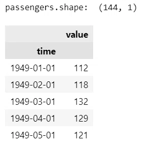
print('passengers.shape: ', passengers.shape)
display(passengers.head())

[Execution Result]
The period (number of rows) is 144 months (12 years) starting from January 1949, and 'value' represents the number of passengers per month.

Data Visualization

We will draw a line graph of the time series.

### 可視化
fig, ax = plt.subplots(figsize=(10, 4))
sns.lineplot(data=passengers, markers='o', ms=5, lw=0.9, legend=False, ax=ax)
ax.set(xlabel='年月', ylabel='月間乗客者数[千人]',
       title='1949－1960年のアメリカ飛行機乗客数')
ax.grid(lw=0.5);

[Execution Result]
An upward 'trend' and a 12-month 'seasonality' are clearly visible!

Let's perform seasonal decomposition and plot the components separately.
We will use statsmodels' seasonal_decompose() for seasonal decomposition.
The period is 12.

### 季節成分の分解

## 季節分解の実行（加法モデル）
result = seasonal_decompose(x=passengers, model='additive', period=12)

## 描画処理
# 描画領域の設定
fig, ax = plt.subplots(4, 1, figsize=(7, 7), sharex=True)
# 原系列の描画
ax[0].plot(result.observed, lw=0.8)
ax[0].set(ylabel='原系列')
ax[0].grid(lw=0.5)
# トレンドの描画
ax[1].plot(result.trend, lw=0.8)
ax[1].set(ylabel='トレンド')
ax[1].grid(lw=0.5)
# 季節調整（周期性）の描画
ax[2].plot(result.seasonal, lw=0.8)
ax[2].set(ylabel='季節調整')
ax[2].grid(lw=0.5)
# 残差の描画
ax[3].plot(result.resid, 'o', ms=5, mec='white', alpha=0.7)
ax[3].axhline(0, color='tab:red', ls='--')
ax[3].set(ylabel='残差')
ax[3].grid(lw=0.5)
plt.tight_layout();

[Execution Result]
We were able to confirm the upward 'trend' and the 12-month 'seasonality'.
It seems necessary to consider a model that accounts for seasonality.
The variation in the residuals seems to contain some remnants of the 12-month cycle.

Dataset Preparation

We will split the data into training and test sets.
For the general time series analysis of the airline passenger data, I referred to the blog of Sales Analytics Inc.
Thank you!

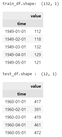
We will split the data into the first 132 months (11 years) for training and the last 12 months (1 year) for testing.

### 学習データとテストデータに分離 1949-1959:学習用, 1960:テスト用

# 前半の132か月を学習用(ts)、最後の12ヶ月をテスト用(ts_test)に分割
train_df = passengers.iloc[:-12]
test_df = passengers.iloc[-12:]

# 分割結果の表示
print('train_df.shape: ', train_df.shape)
display(train_df.head())
print('test_df.shape : ', test_df.shape)
display(test_df.head())

[Execution Result]

We will check the appearance of the training data.
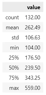
First, we will display the summary statistics.

### 要約統計量の表示
display(train_df.describe().round(2))

[Execution Result]
The minimum value is 104, the maximum is 559, the mean is 262, and the median is 234.

We will draw a time series line graph of the training data.
This corresponds to Figure 7-11 in the text.

### 時系列プロット
fig, ax = plt.subplots(figsize=(10, 4))
sns.lineplot(data=train_df, markers='o', ms=5, lw=0.9, legend=None, ax=ax)
ax.set(xlabel='年月', ylabel='月間乗客者数[千人]',
       title='1949－1959年のアメリカ飛行機乗客数')
ax.grid(lw=0.5)

[Execution Result]

Time Series Data Analysis

Following the analysis procedure in the text, we will grasp the characteristics of the training data time series.

■ Autocorrelation Scatter Plot
We will check the lag-1 autocorrelation using a scatter plot.
This corresponds to Figure 7-12 in the text.

### 散布図の表示

# 相関係数の算出
r = np.corrcoef(train_df.iloc[:-1, 0], train_df.iloc[1:, 0])[0, 1]
# 描画領域の指定
fig, ax = plt.subplots(figsize=(5, 4))
# 散布図の描画 回帰直線付き
sns.regplot(x=train_df[:-1], y=train_df[1:],
            line_kws={'color': 'tomato'},
            scatter_kws={'ec': 'white', 's': 80})
# 修飾
ax.set(xlabel='$y_{t-1}$ [千人]', ylabel='$y_t$ [千人]',
       title=f'ラグ１の散布図\n相関係数:{r:.3f}')
plt.grid(lw=0.5);

[Execution Result]
The horizontal axis is the number of passengers from one month ago, and the vertical axis is the scatter plot of the number of passengers for the current month.

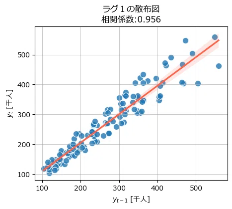
There is a fairly strong positive correlation.
The data points seem to fit the regression line, but there is also a sense that the deviation from the regression line increases once the number exceeds 400.

■ Plotting the Correlogram and Partial Autocorrelation Plot
We will plot the autocorrelation function and the partial autocorrelation function.
The chart of the autocorrelation function is called a correlogram.
Use statsmodels' plot_acf() to draw the correlogram and plot_pacf() to draw the partial autocorrelation function.
This corresponds to Figure 7-13 in the text.

### 自己相関・偏自己相関のプロット

# 描画領域の設定
fig, (ax1, ax2) = plt.subplots(1, 2, figsize=(10, 3))
# コレログラムの描画
plot_acf(train_df, lags=50, ax=ax1, title='コレログラム')
ax1.set(xlabel='Lag', ylabel='ACF', ylim=(-1, 1.2))
ax1.grid(lw=0.5)
# 偏自己相関プロットの描画
plot_pacf(train_df, lags=50, ax=ax2, title='偏自己相関プロット')
ax2.set(xlabel='Lag', ylabel='PACF', ylim=(-1, 1.2))
ax2.grid(lw=0.5)
plt.tight_layout();

[Execution Result]

From the correlogram, a significant autocorrelation function can be seen up to 12 months.
From the partial autocorrelation function, significant values are seen at 1 month ago (lag 1) and 13 months ago (lag 13).
It might be good to consider the first-order difference and the 12th-order difference (first-order difference with a 12-month cycle).

■ Stationarity Test
We will perform an ADF test regarding stationarity.
The null hypothesis is "the data is non-stationary".
We will use adfuller from statsmodels.

### 学習データのADF検定
# 帰無仮説：データは単位根を持つ（非定常である）

# ADF検定（原系列）
adf = adfuller(train_df)
print('原系列　　　:', round(adf[1], 3))

# ADF検定（１階差分列）
adf_diff = adfuller(train_df.diff(1)[1:])
print('１階差分系列:', round(adf_diff[1], 3))

# ADF検定（1階差分&12階差分列）
adf_diff = adfuller(train_df.diff(1).diff(12)[13:])
print('1階&12階系列:', round(adf_diff[1], 3))

[Execution Result]
The p-value of the ADF test result is displayed.

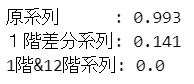
The raw data, or original series, is 99.3%, so it is considered non-stationary (as the null hypothesis cannot be rejected).
The first-order differenced series is 14.1%. Even at a 10% significance level, it is considered non-stationary (as the null hypothesis cannot be rejected).
The first & 12th-order differenced series, obtained by taking a 12th-order difference from the first-order differenced series, is 0.0%, so it is considered stationary (as the null hypothesis can be rejected)!

It seems reasonable to consider the first-order difference and the seasonal first-order difference (12th-order) for the ARIMA model.

Building the SARIMA Model

We will build a SARIMA model that can account for seasonality!

■ Searching for the Optimal Model
Let's use auto_arima from the pmdarima package to automatically search for the optimal order.
By setting the arguments d=1 and D=1, you can specify to take the first-order difference and the seasonal first-order difference.

### auto arima で最適なSARIMAのp,q,P,Qを探索

# 残差の検定
# Ljung-Box検定　：帰無仮説「自己相関関係はない」
# Jarque-Bera検定：帰無仮説「データは正規分布母集団から生成された」

sarima = auto_arima(train_df, seasonal=True, m=12, d=1, D=1)
print(sarima.summary())

[Execution Result]
The optimal model appears to be the SARIMA(1, 1, 0)(0, 1, 0, 12) model.
This is "AR(1) process, 1st-order difference, seasonal 1st-order difference, period 12".
Since it seems MA is not used, it might be a SARI model.

■ Evaluating the Optimal Model
Let's check if the residuals follow a normal distribution using the Jarque-Bera test.
Focus on "Prob(JB)" at the bottom right of the table above.
The p-value "Prob(JB)" of the Jarque-Bera test is 0.75.
Since it is a large value, the null hypothesis cannot be rejected, and it can be interpreted that the residuals "follow a normal distribution" as per the null hypothesis!
Regarding other indicators, the Skew of -0.03 approximates the normal distribution skew of 0, and the Kurtosis of 3.33 approximates the normal distribution kurtosis of 3.
The assumption that the residuals follow a normal distribution seems to be met.

You can use the Ljung-Box test to check for autocorrelation in the residuals.
Focus on "Prob(Q)" at the bottom left of the table above.
The p-value "Prob(Q)" of the Ljung-Box test is 0.89.
Since it is a large value, the null hypothesis cannot be rejected, and as per the null hypothesis, there is "no autocorrelation" in the residuals!

Let's check the state of autocorrelation in the residuals using the correlogram and partial autocorrelation plot.
This corresponds to Figure 7-14 in the text.

### 図7-14 残差のコレログラムの描画

# 残差の取得
resid = sarima.resid()
# 描画領域の設定
fig, (ax1, ax2) = plt.subplots(1, 2, figsize=(10, 3))
# コレログラムの描画
plot_acf(resid, lags=50, ax=ax1, title='コレログラム')
ax1.set(xlabel='Lag', ylabel='ACF', ylim=(-1, 1.2))
ax1.grid(lw=0.5)
# 偏自己相関プロットの描画
plot_pacf(resid, lags=50, ax=ax2, title='偏自己相関プロット')
ax2.set(xlabel='Lag', ylabel='PACF', ylim=(-1, 1.2))
ax2.grid(lw=0.5)
plt.tight_layout();

[Execution Result]
Since there are almost no bars extending outside the blue shaded area,there is no autocorrelation in the residuals!

Let's use the optimal model "sarima" found by auto_arima!

Forecasting for the Test Period

You can forecast for a future period by calling "predict" on "sarima".
In this case, we are forecasting for the next 12 months, so we set the argument n_periods=12.
By the way, there is no need to provide explanatory variables when forecasting.

### 将来24か月の予測
pred = sarima.predict(n_periods=12)
display(pred.to_frame().head())

[Execution Result]
These are the forecasted values for the 12 months of 1960.

Let's visualize the observed values (ground truth) and predicted values for the entire period from 1949 to 1960.
This corresponds to Text Figure 7-15.
The predicted values for the training period can be obtained by applying 'fittedvalues()' to the optimal model 'sarima'.

### 観測値と予測値の時系列プロットの描画

# 描画領域の指定
fig, ax = plt.subplots(figsize=(10, 4))
# 観測値の折れ線グラフの描画
sns.lineplot(data=passengers, markers='o', ms=5, color='tab:blue', lw=0.8,
             legend=None, ax=ax)
# 予測値の折れ線グラフの描画
sns.lineplot(data=sarima.fittedvalues(), color='tab:orange', ls='--', ax=ax)
# 予測値の折れ線グラフの描画
sns.lineplot(data=pred, color='tab:red', ls='--', ax=ax)
# 予測期間の塗りつぶし等
ax.axvline(pd.to_datetime('1960-01-01'), color='black', ls='--', lw=0.5)
ax.axvline(pd.to_datetime('1960-12-01'), color='black', ls='--', lw=0.5)
ax.fill_between([pd.to_datetime('1960-01-01'), pd.to_datetime('1960-12-01')],
                0, 650, color='lightpink', alpha=0.2)
# 修飾
ax.set(xlabel='年月', ylabel='月間乗客者数[千人]', ylim=(0, 650),
       title='1949－1960年のアメリカ飛行機乗客数')
ax.grid(lw=0.5)
# 凡例
ax.plot([], [], '-o', ms=5, lw=0.8, color='tab:blue', label='観測値')
ax.plot([], [], color='tab:orange', ls='--', label='予測値:学習データ')
ax.plot([], [], color='tab:red', ls='--', label='予測値:テストデータ')
ax.legend();

[Execution Result]
The light red area is the test period.
The blue observed values and the red dotted predicted values look quite close!

Executing Anomaly Detection

We are finally in the home stretch!

■ Calculation of Anomaly Score
If the assumption that residuals follow a normal distribution is satisfied, the anomaly score $${a(y_t^{\prime})}$$ can be calculated using the following formula.

$${y_t}$$ is the observed value at time $${t}$$, $${y_t^{\prime}}$$ is the predicted value for $${y_t}$$, and $${\sigma}$$ is the standard deviation of the residuals (more precisely, the standard deviation of the errors).

The text applies the above anomaly score to an ARIMA model.
It is not known whether the above anomaly score can be used for a SARIMA model in the same way.
But I will try using the above anomaly score!

■ Threshold for Anomaly Score
When the assumption that residuals follow a normal distribution is satisfied and there are $${M}$$ explanatory variables,the anomaly score follows a chi-squared distribution with degrees of freedom $${M}$$.
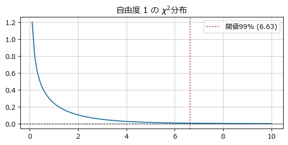
Since this time series data has one explanatory variable, the threshold will be, for example, the 99th percentile (upper 1% point) or the 95th percentile (upper 5% point) of a chi-squared distribution with 1 degree of freedom.

■ Implementation of Anomaly Detection
In this article, I will set the threshold to the 99th percentile (upper 1% point).
Let's check the chi-squared distribution.

### 異常度の閾値に用いたカイ二乗分布の描画

## 設定
# 自由度（変数の数M）
df = 1
# 基準値
pp = 0.99

## カイ二乗分布の確率密度関数と閾値の算出
xval = np.linspace(0, 10, 101)
yval = stats.chi2.pdf(x=xval, df=df)
threshold = stats.chi2.ppf(q=pp, df=df)

## 描画
# 描画領域の設定
plt.figure(figsize=(7, 3))
# カイ二乗分布の確率密度関数の描画
sns.lineplot(x=xval, y=yval)
# 閾値の垂直線の描画
plt.axvline(threshold, color='tab:red', ls=':',
            label=f'閾値{pp:.0%} ({threshold:.2f})')
# y=0の水平線の描画
plt.axhline(0, color='black', lw=0.8, ls='--')
# 修飾
plt.title('自由度 1 の $\chi^2$分布')
plt.grid(lw=0.5)
plt.legend();

[Execution Result]

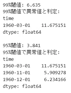
I will calculate the anomaly scores for the test data, calculate the anomaly score threshold, and extract the data points that exceed the threshold.
Following the text, I will calculate the 95th percentile in addition to the 99th percentile.

### 異常検知の実行

## 異常度aの算出
# 学習データの残差の標準偏差の算出
sigma = resid.std(ddof=0)
# テストデータの異常度aの算出 ((実績値-予測値) / 標準偏差)^2
a = ((test_df.value - pred) / sigma)**2

## 異常度の閾値の算出 自由度M=説明変数数のカイ二乗分布の95%点（または99%点）
thres99 = stats.chi2.ppf(q=0.99, df=1)
thres95 = stats.chi2.ppf(q=0.95, df=1)
thres88 = stats.chi2.ppf(q=0.88, df=1)

## 閾値を超える異常度の算出
a_99 = a[a > thres99]
a_95 = a[a > thres95]

## 結果表示
print(f'99%閾値: {thres99:.3f}')
print(f'99%閾値で異常値と判定:\n{a_99}')
print(f'\n95%閾値: {thres95:.3f}')
print(f'95%閾値で異常値と判定:\n{a_95}')

[Execution Result]
At the 99% threshold, March 1960 was identified as an anomaly.

I will visualize the anomaly scores.
This corresponds to Text Figure 7-16.

### 異常度の散布図の描画

# 描画領域の設定
fig, ax = plt.subplots(figsize=(10, 4))
# 異常度aの散布図の描画
sns.scatterplot(x=test_df.index, y=a, s=80, ec='white', alpha=0.7, ax=ax)
# 閾値88%の水平線の描画
ax.axhline(thres88, color='tab:red', lw=0.9, ls='-.',
           label=f'88% ({thres88:.2f})')
# 閾値95%の水平線の描画
ax.axhline(thres95, color='tab:red', lw=0.9, ls='--',
           label=f'95% ({thres95:.2f})')
# 閾値99%の水平線の描画
ax.axhline(thres99, color='tab:red', lw=0.9, ls=':',
           label=f'99% ({thres99:.2f})')
# 修飾
ax.set(xlabel='年月', ylabel='異常度$a$', title='テストデータの異常度プロット')
ax.legend(title='閾値', loc='upper left')
ax.grid(lw=0.5);

[Execution Result]
I visualized the anomaly scores with three thresholds.
If the threshold is set to the 99th percentile, there is one anomalous data point; if set to the 95th percentile, there are three anomalous data points.
It might be possible to perform anomaly detection even if the threshold is set to 88% (just an imaginary musing).

By the way, I am concerned that in March, November, and December 1960,the observed values are smaller than the predicted values!
In other words, it is in a state ofover-prediction.
Did something happen in these three months that caused a decrease in passenger numbers?
Or is 1960 a year where international flights have already become commonplace, and the conventional high growth rate (trend) of passenger numbers is starting to settle down?
I'm curious...

That concludes the detour copying for Chapter 7 ③.

Series Articles

Next Article

Previous Article

Table of Contents

Blog Introduction

I am writing seven series of articles on note. Please take a look!

1. Relaxed Statistics

This is a blog that roughly explores probability and statistics using the Statistical Test Grade 2 problem collection as a guide. Feel free to read it like a casual conversation. Please take a look. It corresponds to the Statistical Test Grade 2 Official Problem Collection CBT version. There is also a distribution of sample code for Python and EXCEL.

2. Experiment! Fun Bayesian Modeling 1 & 2 with PyMC Ver. 5

I will draw and analyze the Bayesian models used in the psychology research of the books 'Fun Bayesian Modeling' and 'Fun Bayesian Modeling 2' using PyMC Ver. 5. Starting with these books, many Bayesian models are written in R language + Stan. I will strive to explore the possibilities of PyMC and make it easy to practice Bayesian modeling. Since these are familiar and easy-to-visualize themes, please try running them with PyMC and let's enjoy it together!

3. Experiment! Iwanami Data Science 1 Bayesian Modeling with PyMC Ver. 5

I will draw and analyze the Bayesian models by four Bayesians from the book 'Experiment! Iwanami Data Science Vol. 1' using PyMC Ver. 5. This book is a good book where you can roughly learn the basics of Bayesian programming. I feel like I have become friends with Bayesian by happily running PyMC models. Everyone, please try running them with PyMC and let's play and learn together!

4. Fun Copying: Bayesian, Python, etc.

I will blog about the results of my 'book copying activities' for Bayesian, Python, and others. I am mainly working on translations into Python. I hope this will serve as sample code for fellow learners who are working on copying.
🍀

5. Introduction to Time Series Analysis for Psychology with R and Stan, using Python and PyMC Ver. 5

I will practice the time series analysis from the book 'Introduction to Time Series Analysis for Psychology with R and Stan' using Python and PyMC Ver. 5. This book is packed with time series analysis themes! I realized the depth of time series analysis. I will happily learn time series analysis with my favorite Python.

6. Writing about Data Science-like Things

I write columns on statistics, data analysis, AI, machine learning, and Python on an irregular basis. There are many articles related to statistics and data science books. Series on 'Statistics', 'Python', 'Mathematics and Python', and 'R' have been created.

7. Python Machine Learning Programming Practice Record

I wrote articles about my various thoughts when I studied the book 'Python Machine Learning Programming: PyTorch & scikit-learn Edition'. This book is a textbook for scikit-learn and PyTorch. If you like, please give it a try.

Thank you very much for reading until the end.