
Bayesian Modeling for Chapter 17 'Comparing Four Tools for Investigating Depression' using PyMC Ver. 5

This article is a statistical documentary depicting the process of "experimentally" implementing the Bayesian model from Chapter 17, 'Comparing Four Tools for Investigating Depression' in the text "Fun Bayesian Modeling 2" using PyMC Ver. 5.
This time, it is a Bayesian analysis with a strong psychological academic tone.
This chapter examines and compares four depression scales using Item Response Theory (IRT).
Thanks to a bit of luck, this PyMC implementation achieved almost the same results as the text! Now, let's enjoy
the world of Bayesian modeling with PyMC!

Please refer to the linked article for the introduction of the text, citation notation, series preface, and version information for PyMC, etc.
The data used in the text, along with sample scripts for R, Stan, etc., can be obtained by downloading them from the publisher's website.
Summary
Overview of the text
Authors: Dr. Naoya Todo, Dr. Yusuke Umegaki
Model Difficulty: ★★★★★ (Difficult)
Self-Evaluation
Rating
$$
\begin{array}{c:c:c}
Implementation Accuracy & ★★★★★ & GoooD! \\
Result Reproducibility & ★★★★★ & Best✨ \\
Fun & ★★★★★ & Fun! \\
\end{array}
$$

Evaluation Points
I defeated the nemesis 'Ordered' constraint!
This Bayesian model imposes an Ordered constraint (in ascending order of values) on the 2D variable $${\kappa}$$.
In previous Bayesian modeling attempts, I couldn't implement the Ordered constraint for 2D variables and must have cried myself to sleep many times...
This time, regardless of whether it made sense, I mimicked the official PyMC sample code and set the arguments, and although I don't understand the principle, the Ordered constraint worked in the row direction! Yay!
Efforts, Joys, and Reflections
Continuing from last time, 'Factor Analysis' appeared again!
It seems I need to properly face factor analysis sometime, somewhere.
This time, I used Confirmatory Factor Analysis from semopy.

Model Overview
Overview of the text's research and experiments
■ Analysis Overview
We perform Bayesian modeling on the characteristics of four self-report depression measurement scales for university students using a mathematical model based on Item Response Theory.
■ Data Overview
This is response data obtained from an online survey of 824 Japanese university students.
■ List of Scales Analyzed
$$
\begin{array}{l:l:l:l}
Scale Name & Overview & Score & Reverse Items\\
\hline
SDS & 20 items, 4-point scale & 1 to 4 points & 10 items \\
CES-D & 20 items, 4-point scale & 0 to 3 points & 4 items\\
BDI-II & 21 items, 4 or 7-point scale & 0 to 3 points & None \\
PHQ-9 & 9 items, 4-point scale & 0 to 3 points & None \\
\end{array}
$$
The scores are values converted from the response values to the questionnaire items.
For example, if the score is '1 to 4 points' on a 4-point scale, there are 4 levels of response values, which are scored from 1 to 4.
In the case of the 7-point scale for BDI-II, it is said that the 7 levels of response values are scored in the range of 0 to 3 points.
The analysis overview is illustrated below.

Text Modeling
■ Objective Variables and Parameters of Interest
The objective variable is the response value $${U_{ij}}$$ for item $${j}$$ by respondent $${i}$$.
Parameters of interest include depression level $${{\theta_i}}$$, discrimination parameter $${a_{j}}$$, discrimination parameter $${{\times}}$$ category difficulty parameter $${{\kappa_{jk}}}$$, and test information and relative efficiency calculated from these parameters.
■ Mathematical Model
This is a mathematical model based on Item Response Theory.
When the depression level of respondent $${i}$$ is $${{\theta_i}}$$, the probability $${P_{jk}(\theta_i)}$$ of responding with category (likely score) $${k}$$ for (question) item $${j}$$ is defined.
$$
\begin{align*}
P_{jk}(\theta_i) &= P^{+}_{jk}(\theta_i) - P^{+}_{j(k+1)}(\theta_i) \\
P^{+}_{jk}(\theta_i) &= \cfrac{1}{1 + \exp(-a_j(\theta_i - b_{jk}))} = \cfrac{1}{1 + \exp(-a_j \theta_i + \kappa_{jk})} \\
\end{align*}
$$
【Overview of Variables and Symbols】
$${P^{+}_{jk}(\theta_i)}$$ is the probability that respondent $${i}$$ answers category $${k}$$ or higher for item $${j}$$
$${a_{j}}$$ is the discrimination parameter
$${\kappa_{jk}}$$ is the discrimination parameter $${{\times}}$$ category difficulty parameter
■ Bayesian Model
Since the likelihood function is not included in the text, I will write it by reverse-engineering the Stan code.
$$
\begin{align*}
U_{ij} &\sim \text{OrderedLogistic}\ (a_j \theta_i,\ \kappa_{jk}) \\
\theta_i &\sim \text{Normal}\ (0,\ 1) \\
a_j &\sim \text{LogNormal}\ (0,\ 2) \\
\kappa_{jk} &\sim \text{Normal}\ (0,\ 10^2) \\
\end{align*}
$$
【Overview of Variables and Symbols】
$${U_{ij}}$$ is the response value for item $${j}$$ by respondent $${i}$$.
OrderedLogistic is an ordered logistic distribution, where the first argument is the predictor and the second argument is the cutpoints.
The second argument of the Normal distribution $${{\text{Normal}}}$$ is the variance.
The second argument of the LogNormal distribution $${{\text{LogNormal}}}$$ is the standard deviation.

■ Analysis and Analysis Results
I believe the descriptions of the analysis methods and numerical values in the text are accurate, so I recommend reading the text.
Please see the 'PyMC Implementation' chapter for analysis using inferred values from my own PyMC model.
PyMC Implementation
Let's enjoy PyMC & Python !
Preparation and data verification
1. Import
### インポート

# 数値・確率計算
import pandas as pd
import numpy as np
import pingouin as pg

# PyMC
import pymc as pm
import arviz as az

# 確認的因子分析
import semopy

# 描画
import matplotlib.pyplot as plt
import seaborn as sns
plt.rcParams['font.family'] = 'Meiryo'

# ユーティリティ
import pickle

# ワーニング表示の抑制
import warnings
warnings.simplefilter('ignore')
2. Data loading and preprocessing
Load the CSV file "4scale_data.csv" into a pandas DataFrame.
### データの読み込み
data_orgn = pd.read_csv('4scale_data.csv')
display(data_orgn)
[Execution result]
Data with 824 rows and 70 columns.
Rows represent individual respondents.
Columns are combinations of scale names and item numbers.
Values are the scores (respondent answers) for each scale and item.

Process the data.
First, convert from wide format to long format.
### データ前処理:データを縦持ちに変換

## 設定
# 尺度のリスト
methods = ['SDS', 'CESD', 'BDI', 'PHQ9']

## dataを縦持ちに変換
# dataのコピー、旧indexを残す(回答者IDにする)
data = data_orgn.copy().reset_index()
# 縦持ちに変換、variableに「尺度+番号」がセットされる
data = pd.melt(data, id_vars=['index'], value_vars=data.columns)
# 「尺度+番号」から尺度を切り抜き(尺度リストから一致する尺度名を取り出してセット)
data['shaku'] = (data['variable']
                .apply(lambda x: [m for m in methods if x[:3] in m][0]))
# 「尺度+番号」から番号を切り抜き(shakuにセットした尺度名を''に置換して整数型へ)
data['ban'] = (data[['variable', 'shaku']]
               .apply(lambda x: int(x[0].replace(x[1], '')), axis=1))
# 列の絞り込みと列名の変更
data = data[['index', 'shaku', 'ban', 'value']]
data.columns = ['回答者ID', '尺度', '項目番号', '得点']
# データフレームの表示
display(data)
[Execution result]
The format is now score data by respondent ID, scale, and item number.

Next, create total score data by scale and respondent ID.
### データ前処理:尺度・回答者IDごとの合計得点のデータフレームの作成
data_sum = data.groupby(by=['尺度', '回答者ID'])['得点'].sum().reset_index()
display(data_sum)
[Execution result]
How to read the table:
The total score for the BDI scale by respondent ID 0 is 1.


Descriptive statistics and confirmatory factor analysis
The text presents a rigorous analytical procedure to the reader.
I will do my best to follow the analytical procedure!
I will trace the analytical procedures in Section 17.2.1 "Descriptive Statistics" and Section 17.2.2 "Correlation Coefficients between Scale Scores and Factors" of the text.
1. Descriptive statistics
■ Mean and standard deviation of total scores
Calculate the mean and standard deviation of the total scores for each scale.
In the text, this is described in the text on page 188.
### 記述統計:各尺度の尺度得点について平均・標準偏差の算出 ※テキスト188ページ

# 尺度ごとに合計得点の平均と標準偏差を算出、methodsリスト順に行をソート
stats_df01 = (data_sum.groupby(['尺度'])['得点'].agg(['mean', 'std'])
              .reindex(methods))
display(stats_df01.round(2))
[Execution result]

■ Distribution of depression levels
Next is the distribution (number of people) of depression levels.
It uses the groupings (cutoff points) proposed in previous studies.
In the text, this is described in the text on pages 188-189.
### 記述統計:抑うつ度の分布(人数)の算出 ※テキスト188~189ページ

# CESD 閾値15
tmp = data_sum[data_sum['尺度']=='CESD']
CESDn = (tmp['得点'] <= 15).sum()       # 非抑うつ
CESDp = (tmp['得点'] > 15).sum()        # 抑うつ
print(f'CESD: 非抑うつ{CESDn}名, 抑うつ{CESDp}名')

# PHQ9 閾値9
tmp = data_sum[data_sum['尺度']=='PHQ9']
PHQ9n = (tmp['得点'] <= 9).sum()        # 非抑うつ
PHQ9p = (tmp['得点'] > 9).sum()         # 抑うつ
print(f'PHQ9: 非抑うつ{PHQ9n}名, 抑うつ{PHQ9p}名')

# SDS 閾値47, 55
tmp = data_sum[data_sum['尺度']=='SDS']
SDSl = (tmp['得点'] <= 47).sum()        # 軽度/非抑うつ
SDSm = ((tmp['得点'] > 47) & (tmp['得点'] <= 55)).sum()   # 中程度
SDSh = (tmp['得点'] > 55).sum()         # 重度
print(f'SDS : 軽度/非抑うつ{SDSl}名, 中程度{SDSm}名, 重度{SDSh}名')

# BDI 閾値13, 19, 28
tmp = data_sum[data_sum['尺度']=='BDI']
BDIn = (tmp['得点'] <= 13).sum()        # 非抑うつ
BDIl = ((tmp['得点'] > 13) & (tmp['得点'] <= 19)).sum()   # 軽度
BDIm = ((tmp['得点'] > 19) & (tmp['得点'] <= 28)).sum()   # 中程度
BDIh = (tmp['得点'] > 28).sum()         # 重度
print(f'BDI : 非抑うつ{BDIn}名, 軽度{BDIl}名, 中程度{BDIm}名, 重度{BDIh}名')
[Execution result]

■ Alpha coefficient of scale scores
Next is the alpha coefficient for the scale scores of each scale.
This is a statistic called Cronbach's alpha coefficient.
Use the cronbach_alpha() function from the pingouin library.
In the text, this is described in the text on page 189.
### 記述統計:各尺度の尺度得点の信頼性係数α(クロンバックのα係数)の算出
# ※テキスト189ページ, pingouinのcronbach_alpha()でクロンバックのα係数を算出

# 結果を格納するデータフレームの初期化
stats_df02 = pd.DataFrame()
# 各尺度ごとにα係数を算出してデータフレームに追加する処理を繰り返す
for method in methods:
    # α係数と信頼区間の算出 pingouinのcronbach_alpha()
    alpha, ci = pg.cronbach_alpha(data[data['尺度']==method],
                                  items='項目番号', subject='回答者ID',
                                  scores='得点', ci=0.95)
    # データフレームに追加
    stats_df02 = pd.concat([stats_df02,
                            pd.DataFrame({method: [alpha, ci[0], ci[1]]})],
                           axis=1)
# データフレームの縦横を変換して列名をセット
stats_df02 = stats_df02.set_axis(['α', '2.5%CI', '97.5%CI']).T
# データフレームの表示
display(stats_df02.round(2))
[Execution result]
According to the text, "these scale scores were considered to have sufficient reliability."


2. Correlation coefficients between scale scores and factors
The text proceeds to confirmatory factor analysis, assuming one factor (a latent variable representing the degree of depression) behind each scale and assuming correlations between the factors of each scale.
■ Correlation coefficients between scale scores
First, calculate the correlation coefficient $${r}$$ between scale scores.
Calculate the correlation coefficient using the pandas corr() function.
In the text, this is described in the text on page 189.
### 尺度得点間の相関係数の算出 ※テキスト189ページ

# 行:回答者ID、列:尺度、値:得点のデータフレームを作成
data_sum2 = (data_sum.pivot_table(index='回答者ID', columns='尺度', values='得点')
             .reset_index(drop=True))
data_sum2.columns.name = None
# display(data_sum2)

# 尺度得点間の相関係数:corr()を算出して表示
display(data_sum2.corr().round(2))
[Execution result]
As stated in the text, a strong positive correlation of $${r=0.68-0.81}$$ is observed between the scale scores.

■ Confirmatory Factor Analysis: Correlations between depression factors
I will attempt a confirmatory factor analysis using the semopy library (my first time).
For the implementation of confirmatory factor analysis using semopy, I referred to the blog of Kosuke Fukunaka.
Thank you!
Executing confirmatory factor analysis.
### 確認的因子分析の実行
# semopyを利用
# 参考サイト:https://note.com/k_fukunaka/n/ncf493169157a

# 確認的因子分析モデルの定義
desc = """
        PHQ9 =~ PHQ91 + PHQ92 + PHQ93 + PHQ94 + PHQ95 + PHQ96 + PHQ97 + PHQ98 \
                + PHQ99
        CESD =~ CESD1 + CESD2 + CESD3 + CESD4 + CESD5 + CESD6 + CESD7 + CESD8 \
                + CESD9 + CESD10 + CESD11 + CESD12 + CESD13 + CESD14 + CESD15 \
                + CESD16 + CESD17 + CESD18 + CESD19 + CESD20
        SDS =~ SDS1 + SDS2 + SDS3 + SDS4 + SDS5 + SDS6 + SDS7 + SDS8 + SDS9 \
               + SDS10 + SDS11 + SDS12 + SDS13 + SDS14 + SDS15 + SDS16 + SDS17 \
               + SDS18 + SDS19 + SDS20
        BDI =~ BDI1 + BDI2 + BDI3 + BDI4 + BDI5 + BDI6 + BDI7 + BDI8 + BDI9 \
               + BDI10 + BDI11 + BDI12 + BDI13 + BDI14 + BDI15 + BDI16 + BDI17 \
               + BDI18 + BDI19 + BDI20 + BDI21
        """

# 確認的因子分析の実行
model_cfa = semopy.Model(desc)
result_cfa = model_cfa.fit(data_orgn)
[Execution Result] None
Checking the 'goodness of fit' of the confirmatory factor analysis.
In the text, this is described in text on page 189.
### 確認的因子分析の結果:適合度の確認 ※テキスト189ページ
# 適合度検定の結果:chi2 p-value 0.000,  RMSEA 0.075
stats_df03 = semopy.calc_stats(model_cfa)
display(stats_df03.T.round(3))
[Execution Result]
The p-value for the goodness-of-fit test is 0.000 for 'chi2 p-value'. It is significant at the 1% level.
RMSEA is 0.075 for 'RMSEA'. This is considered to be the same value as the 0.8 in the text.

I will explore the correlations between factors.
In the text, this is described in text on page 189.
I am not entirely sure about the calculation method, so the appropriateness of the following code is unknown.
Also, the calculated correlation coefficients differ from those in the text.
### 構成概念スコアの推定 ※テキスト189ページ 因子間に強い正の相関 r=0.82-0.91
# ★因子間の相関係数の算出方法がこれで良いのか不明・・・

# 因子スコアの推定の実行
factor_score = model_cfa.predict_factors(data_orgn)
# 結果表示
print('因子スコアの推定結果')
display(factor_score)
# 因子スコアの相関関係の算出
print('因子スコア間の相関関係')
display(factor_score.corr().round(3))
[Execution Result]
I measured the correlation coefficients against the predicted values of the factor scores.

If I were to write it in the style of the text, it would be "$${r=0.90-0.97}$$".
The values are higher than the "$${r=0.82-0.91}$$" in the text.
Below, I will leave the results of the confirmatory factor analysis as a record.
■ Results of Confirmatory Factor Analysis: Summary of the four factors
### 確認的因子分析の結果:4つの因子の結果表示
# Est.Stdは標準偏回帰係数
inspect_cfa = model_cfa.inspect(std_est=True)
display(inspect_cfa.iloc[70:80].round(3))
[Execution Result]

■ Path Diagram
I will save the path diagram image file to the working folder with the filename 'model_cfa.png'.
### 確認的因子分析の結果:推定後のパス係数付きパス図の出力
# 共分散を表示する、標準化係数を表示する
g = semopy.semplot(model_cfa, 'model_cfa.png', plot_covs=True, std_ests=True)
display(g)
[Execution Result]

This concludes the various analyses before the Bayesian analysis.

Building the Bayesian model
I will create four models by scale, but except for the fact that the analysis target data is different, the content of the models is all the same.
Mathematical expression of the model
This is a 'pseudo-mathematical' notation of the PyMC model I am aiming for.
$$
\begin{align*}
\alpha &\sim \text{LogNormal}\ (\text{mu}=0,\ \text{sigma}=2,\ \text{dims}=item) \\
\kappa &\sim \text{Normal} (\text{mu}=[-0.1, 0, 0.1], \text{sigma}=10,\ \text{ordered},\ \text{dims}=(item,\ cutpoint)) \\
\theta &\sim \text{Normal}\ (\text{mu}=0,\ \text{sigma}=1,\ \text{dims}=id) \\
likelihood &\sim \text{OrderedLogistic}\ (\text{eta}=\alpha[itemIdx] \times \theta[idIdx],\ \text{cutpoints}=\kappa[itemIdx, :\ ]) \\
\end{align*}
$$
Now, I will create a Bayesian model for each of the four scales.
1. SDS
(1) Model definition
We describe the model faithfully to the mathematical expression.
### モデルの定義:SDS

## データの準備:分析対象尺度の抽出
# 尺度SDSのデータを抽出
data_in = data[data['尺度']=='SDS'].reset_index(drop=True)
# 項目番号のインデックス化(0始まりにする)
data_in['項目番号'] = data_in['項目番号'] - 1
# 項目番号の要素数
num_item = data_in['項目番号'].nunique()
# 得点の範囲を0~3に揃える:SDSのみの処理
data_in['得点'] = data_in['得点'] - 1
# 得点の要素数
num_score = data_in['得点'].nunique()

## モデルの定義
with pm.Model() as model_sds:

    ### coordの定義
    # データのインデックス
    model_sds.add_coord('data', values=data_in.index, mutable=True)
    # 回答者ID  stan:N, i
    model_sds.add_coord('id', values=sorted(data_in['回答者ID'].unique()),
                        mutable=True)
    # 項目番号  stan:J, j
    model_sds.add_coord('item', values=sorted(data_in['項目番号'].unique()),
                        mutable=True)
    # カットポイント  stan:3
    model_sds.add_coord('cutpoint', values=list(range(num_score - 1)),
                        mutable=True)

    ### dataの定義
    # 目的変数:得点U_ij
    y = pm.ConstantData('y', value=data_in['得点'].values, dims='data')
    # 回答者IDのインデックス
    idIdx = pm.ConstantData('idIdx', value=data_in['回答者ID'].values,
                            dims='data')
    # 項目番号のインデックス
    itemIdx = pm.ConstantData('itemIdx', value=data_in['項目番号'].values,
                              dims='data')

    ### 事前分布
    ## a_j = 識別力母数
    alpha = pm.LogNormal('alpha', mu=0, sigma=2, dims='item')
    ## κ_jk = 識別力母数α_j × カテゴリ困難度母数b_jk
    #  ※muにcutpointの数(3)のパラメータを指定したら行単位のorederdが効いた
    kappa = pm.Normal('kappa', mu=[-0.1, 0, 0.1], sigma=10,
                      dims=('item', 'cutpoint'),
                      transform=pm.distributions.transforms.ordered)
    ## θ_i = 抑うつ度
    theta = pm.Normal('theta', mu=0, sigma=1, dims='id')

    ### 尤度:順序ロジスティック分布
    likelihood = pm.OrderedLogistic('likelihood',
                                    eta=alpha[itemIdx] * theta[idIdx],
                                    cutpoints=kappa[itemIdx, :],
                                    compute_p=False,
                                    observed=y, dims='data')
[Model annotations]
-
Defining coords
You can name coordinates and set the values they can take.
This time, we set the following four.Data row coordinates: name 'data', value 'row index'
Respondent coordinates: name 'id', value 'respondent ID'
Item number coordinates: name 'item', value 'item number'
Cutpoint coordinates: name 'cutpoint', value 'scale score (excluding maximum score)'
Coordinates for elements of the factor loading matrix to be freely estimated: name 'Z1', value 'Z1 index'
-
Defining data
We set the following three.Score: y (target variable, respondent's answer value)
Respondent ID index: idIdx
Item number index: itemIdx
-
Prior distribution of parameters
It follows the mathematical expression of the model.
-
Ordered constraint for $${\kappa}$$
When I provided three values (the number of cutpoints) in ascending order to the mean parameter of the normal distribution, the ordered constraint specified in the transform argument worked!
-
Likelihood
It is an ordered logistic distribution.
(2) Checking the model structure
### モデルの表示
model_sds
[Execution result]
It is a simple structure.

### モデルの可視化
pm.model_to_graphviz(model_sds)
[Execution result]

(3) Sampling from the posterior distribution
The number of random number generations is smaller than in the text.
By setting nuts_sampler='numpyro', you can use numpyro as the NUTS sampler.
The processing time was approximately 10 minutes.
### 事後分布からのサンプリング ※NUTSサンプラーにnumpyroを使用 10分20秒
# テキスト: iter=2000, warmup=?, chains=4
with model_sds:
    idata_sds = pm.sample(draws=1000, tune=1000, chains=4, target_accept=0.8,
                          nuts_sampler='numpyro', random_seed=1234)
[Execution result] Omitted
(4) Checking the sampled data
Check $${\hat{R}}$$ and the trace plot.
The convergence check for the posterior distribution is set to $${\hat{R} \leq 1.1}$$.
Here, I will confirm that there are no parameters with $${\hat{R} > 1.01}$$.
### r_hat>1.1の確認
# 設定
idata_in = idata_sds      # idata名
threshold = 1.01          # しきい値

# しきい値を超えるR_hatの個数を表示
(az.rhat(idata_in) > threshold).sum()
[Execution result]
There were 0 parameters with $${\hat{R} > 1.01}$$.
I was able to confirm that all parameters satisfy $${\hat{R} \leq 1.1}$$.

I will roughly check the summary statistics and trace plot of the posterior distribution sampling data.
### 推論データの要約統計情報の表示
pm.summary(idata_sds, hdi_prob=0.95, round_to=3)
[Execution result]

I will check the state of the posterior distribution sampling data using a trace plot.
Only some parameters are displayed.
### トレースプロットの表示
pm.plot_trace(idata_sds, compact=False)
plt.tight_layout();
[Execution result]
From the graph on the left, it can be seen that the four Markov chains have almost the same distribution.
In the graph on the right, the lines are drawn evenly.
It appears to have converged.

(5) Saving inference data
Let's save it to a file in case we (might) reuse the inference data.
Save idata_sds using pickle.
### idataの保存 pickle
file = r'idata_sds_ch17.pkl'
with open(file, 'wb') as f:
    pickle.dump(idata_sds, f)
The code for loading is as follows.
### idataの読み込み pickle
file = r'idata_sds_ch17.pkl'
with open(file, 'rb') as f:
    idata_sds_load = pickle.load(f)
2. CES-D
(1) Defining the model
I will describe the model faithfully to the mathematical expression.
### モデルの定義:CESD

## データの準備:分析対象尺度の抽出
# 尺度CESDのデータを抽出
data_in = data[data['尺度']=='CESD'].reset_index(drop=True)
# 項目番号のインデックス化(0始まりにする)
data_in['項目番号'] = data_in['項目番号'] - 1
# 項目番号の要素数
num_item = data_in['項目番号'].nunique()
# 得点の範囲を0~3に揃える:SDSのみの処理
# data_in['得点'] = data_in['得点'] - 1
# 得点の要素数
num_score = data_in['得点'].nunique()

## モデルの定義
with pm.Model() as model_cesd:

    ### coordの定義
    # データのインデックス
    model_cesd.add_coord('data', values=data_in.index, mutable=True)
    # 回答者ID  stan:N, i
    model_cesd.add_coord('id', values=sorted(data_in['回答者ID'].unique()),
                        mutable=True)
    # 項目番号  stan:J, j
    model_cesd.add_coord('item', values=sorted(data_in['項目番号'].unique()),
                        mutable=True)
    # カットポイント  stan:3
    model_cesd.add_coord('cutpoint', values=list(range(num_score - 1)),
                        mutable=True)

    ### dataの定義
    # 目的変数:得点U_ij
    y = pm.ConstantData('y', value=data_in['得点'].values, dims='data')
    # 回答者IDのインデックス
    idIdx = pm.ConstantData('idIdx', value=data_in['回答者ID'].values,
                            dims='data')
    # 項目番号のインデックス
    itemIdx = pm.ConstantData('itemIdx', value=data_in['項目番号'].values,
                              dims='data')

    ### 事前分布
    ## a_j = 識別力母数
    alpha = pm.LogNormal('alpha', mu=0, sigma=2, dims='item')
    ## κ_jk = 識別力母数α_j × カテゴリ困難度母数b_jk
    #  ※muにcutpointの数(3)のパラメータを指定したら行単位のorederdが効いた
    kappa = pm.Normal('kappa', mu=[-0.1, 0, 0.1], sigma=10,
                      dims=('item', 'cutpoint'),
                      transform=pm.distributions.transforms.ordered)
    ## θ_i = 抑うつ度
    theta = pm.Normal('theta', mu=0, sigma=1, dims='id')

    ### 尤度:順序ロジスティック分布
    likelihood = pm.OrderedLogistic('likelihood',
                                    eta=alpha[itemIdx] * theta[idIdx],
                                    cutpoints=kappa[itemIdx, :],
                                    compute_p=False,
                                    observed=y, dims='data')
[Model annotation] Omitted
(2) Checking the model structure
### モデルの表示
model_cesd
[Execution result]

### モデルの可視化
pm.model_to_graphviz(model_cesd)
[Execution Results]

(3) Sampling from the posterior distribution
The number of random number generations is smaller than in the text.
By setting nuts_sampler='numpyro', you can use numpyro as the NUTS sampler.
The processing time was approximately 3 minutes.
### 事後分布からのサンプリング ※NUTSサンプラーにnumpyroを使用 3分
# テキスト: iter=2000, warmup=?, chains=4
with model_cesd:
    idata_cesd = pm.sample(draws=1000, tune=1000, chains=4, target_accept=0.9,
                           nuts_sampler='numpyro', random_seed=1234)
[Execution Results] Omitted
(4) Confirmation of sampling data
Check $$\hat{R}$$ and the trace plot.
The convergence check for the posterior distribution is set to $$\hat{R} \leq 1.1$$.
Here, we confirm that there are no parameters with $$\hat{R} > 1.01$$.
### r_hat>1.1の確認
# 設定
idata_in = idata_cesd     # idata名
threshold = 1.01          # しきい値

# しきい値を超えるR_hatの個数を表示
print((az.rhat(idata_in) > threshold).sum())
[Execution Results]
There were 0 parameters with $$\hat{R} > 1.01$$.
We were able to confirm that all parameters satisfy $$\hat{R} \leq 1.1$$.

We will roughly check the summary statistics and trace plots of the posterior distribution sampling data.
### 推論データの要約統計情報の表示
pm.summary(idata_cesd, hdi_prob=0.95, round_to=3)
[Execution Results]

We will check the state of the posterior distribution sampling data using trace plots.
The display is limited to some parameters.
### トレースプロットの表示
pm.plot_trace(idata_cesd, compact=False)
plt.tight_layout();
[Execution Results]
From the graph on the left, it can be seen that the four Markov chains have almost the same distribution.
In the graph on the right, the lines are drawn evenly.
It is considered to have converged.

(5) Saving inference data
Let's save it to a file in case we (might) reuse the inference data.
Save idata_cesd using pickle.
### idataの保存 pickle
file = r'idata_cesd_ch17.pkl'
with open(file, 'wb') as f:
    pickle.dump(idata_cesd, f)
The code for loading is as follows.
### idataの読み込み pickle
file = r'idata_cesd_ch17.pkl'
with open(file, 'rb') as f:
    idata_cesd_load = pickle.load(f)
3. BDI-II
(1) Model definition
We describe the model faithfully to the mathematical expression.
### モデルの定義:BDI

## データの準備:分析対象尺度の抽出
# 尺度BDIのデータを抽出
data_in = data[data['尺度']=='BDI'].reset_index(drop=True)
# 項目番号のインデックス化(0始まりにする)
data_in['項目番号'] = data_in['項目番号'] - 1
# 項目番号の要素数
num_item = data_in['項目番号'].nunique()
# 得点の範囲を0~3に揃える:SDSのみの処理
# data_in['得点'] = data_in['得点'] - 1
# 得点の要素数
num_score = data_in['得点'].nunique()

## モデルの定義
with pm.Model() as model_bdi:

    ### coordの定義
    # データのインデックス
    model_bdi.add_coord('data', values=data_in.index, mutable=True)
    # 回答者ID  stan:N, i
    model_bdi.add_coord('id', values=sorted(data_in['回答者ID'].unique()),
                        mutable=True)
    # 項目番号  stan:J, j
    model_bdi.add_coord('item', values=sorted(data_in['項目番号'].unique()),
                        mutable=True)
    # カットポイント  stan:3
    model_bdi.add_coord('cutpoint', values=list(range(num_score - 1)),
                        mutable=True)

    ### dataの定義
    # 目的変数:得点U_ij
    y = pm.ConstantData('y', value=data_in['得点'].values, dims='data')
    # 回答者IDのインデックス
    idIdx = pm.ConstantData('idIdx', value=data_in['回答者ID'].values,
                            dims='data')
    # 項目番号のインデックス
    itemIdx = pm.ConstantData('itemIdx', value=data_in['項目番号'].values,
                              dims='data')

    ### 事前分布
    ## a_j = 識別力母数
    alpha = pm.LogNormal('alpha', mu=0, sigma=2, dims='item')
    ## κ_jk = 識別力母数α_j × カテゴリ困難度母数b_jk
    #  ※muにcutpointの数(3)のパラメータを指定したら行単位のorederdが効いた
    kappa = pm.Normal('kappa', mu=[-0.1, 0, 0.1], sigma=10,
                      dims=('item', 'cutpoint'),
                      transform=pm.distributions.transforms.ordered)
    ## θ_i = 抑うつ度
    theta = pm.Normal('theta', mu=0, sigma=1, dims='id')

    ### 尤度:順序ロジスティック分布
    likelihood = pm.OrderedLogistic('likelihood',
                                    eta=alpha[itemIdx] * theta[idIdx],
                                    cutpoints=kappa[itemIdx, :],
                                    compute_p=False,
                                    observed=y, dims='data')
[Model Annotations] Omitted
(2) Confirmation of model appearance
### モデルの表示
model_bdi
[Execution Results]

### モデルの可視化
pm.model_to_graphviz(model_cesd)
[Execution Results]

(3) Sampling from the posterior distribution
The number of random number generations is smaller than in the text.
By setting nuts_sampler='numpyro', you can use numpyro as the NUTS sampler.
The processing time was approximately 4 minutes.
### 事後分布からのサンプリング ※NUTSサンプラーにnumpyroを使用 4分20秒
# テキスト: iter=2000, warmup=?, chains=4
with model_bdi:
    idata_bdi = pm.sample(draws=1000, tune=1000, chains=4, target_accept=0.9,
                           nuts_sampler='numpyro', random_seed=1234)
[Execution Results] Omitted
(4) Confirmation of sampling data
Check $$\hat{R}$$ and the trace plot.
The convergence check for the posterior distribution is set to $$\hat{R} \leq 1.1$$.
Here, we confirm that there are no parameters with $$\hat{R} > 1.01$$.
### r_hat>1.1の確認
# 設定
idata_in = idata_bdi      # idata名
threshold = 1.01          # しきい値

# しきい値を超えるR_hatの個数を表示
print((az.rhat(idata_in) > threshold).sum())
[Execution Result]
There were 0 parameters with $$\hat{R} > 1.01$$.
We were able to confirm that all parameters satisfy $$\hat{R} \leq 1.1$$.

We will roughly check the summary statistics and trace plots of the posterior distribution sampling data.
### 推論データの要約統計情報の表示
pm.summary(idata_bdi, hdi_prob=0.95, round_to=3)
[Execution Result]

We will check the state of the posterior distribution sampling data using trace plots.
Only a subset of parameters is displayed.
### トレースプロットの表示
pm.plot_trace(idata_bdi, compact=False)
plt.tight_layout();
[Execution Result]
From the graph on the left, it can be seen that the four Markov chains have almost the same distribution.
In the graph on the right, the lines are drawn evenly.
It is considered to have converged.

(5) Saving inference data
Let's save the inference data to a file in case we (might) reuse it.
We will save idata_bdi using pickle.
### idataの保存 pickle
file = r'idata_bdi_ch17.pkl'
with open(file, 'wb') as f:
    pickle.dump(idata_bdi, f)
The code for loading is as follows.
### idataの読み込み pickle
file = r'idata_bdi_ch17.pkl'
with open(file, 'rb') as f:
    idata_bdi_load = pickle.load(f)
4. PHQ-9
(1) Model definition
We will describe the model faithfully to the mathematical expression.
### モデルの定義:PHQ9

## データの準備:分析対象尺度の抽出
# 尺度PHQ9のデータを抽出
data_in = data[data['尺度']=='PHQ9'].reset_index(drop=True)
# 項目番号のインデックス化(0始まりにする)
data_in['項目番号'] = data_in['項目番号'] - 1
# 項目番号の要素数
num_item = data_in['項目番号'].nunique()
# 得点の範囲を0~3に揃える:SDSのみの処理
# data_in['得点'] = data_in['得点'] - 1
# 得点の要素数
num_score = data_in['得点'].nunique()

## モデルの定義
with pm.Model() as model_phq9:

    ### coordの定義
    # データのインデックス
    model_phq9.add_coord('data', values=data_in.index, mutable=True)
    # 回答者ID  stan:N, i
    model_phq9.add_coord('id', values=sorted(data_in['回答者ID'].unique()),
                         mutable=True)
    # 項目番号  stan:J, j
    model_phq9.add_coord('item', values=sorted(data_in['項目番号'].unique()),
                         mutable=True)
    # カットポイント  stan:3
    model_phq9.add_coord('cutpoint', values=list(range(num_score - 1)),
                         mutable=True)

    ### dataの定義
    # 目的変数:得点U_ij
    y = pm.ConstantData('y', value=data_in['得点'].values, dims='data')
    # 回答者IDのインデックス
    idIdx = pm.ConstantData('idIdx', value=data_in['回答者ID'].values,
                            dims='data')
    # 項目番号のインデックス
    itemIdx = pm.ConstantData('itemIdx', value=data_in['項目番号'].values,
                              dims='data')

    ### 事前分布
    ## a_j = 識別力母数
    alpha = pm.LogNormal('alpha', mu=0, sigma=2, dims='item')
    ## κ_jk = 識別力母数α_j × カテゴリ困難度母数b_jk
    #  ※muにcutpointの数(3)のパラメータを指定したら行単位のorederdが効いた
    kappa = pm.Normal('kappa', mu=[-0.1, 0, 0.1], sigma=10,
                      dims=('item', 'cutpoint'),
                      transform=pm.distributions.transforms.ordered)
    ## θ_i = 抑うつ度
    theta = pm.Normal('theta', mu=0, sigma=1, dims='id')

    ### 尤度:順序ロジスティック分布
    likelihood = pm.OrderedLogistic('likelihood',
                                    eta=alpha[itemIdx] * theta[idIdx],
                                    cutpoints=kappa[itemIdx, :],
                                    compute_p=False,
                                    observed=y, dims='data')
[Model Annotation] Omitted
(2) Checking the model structure
### モデルの表示
model_phq9
[Execution Result]

### モデルの可視化
pm.model_to_graphviz(model_phq9)
[Execution Result]

(3) Sampling from the posterior distribution
The number of random number generations is smaller than in the text.
By setting nuts_sampler='numpyro', you can use numpyro as the NUTS sampler.
The processing time was approximately 1 minute.
### 事後分布からのサンプリング ※NUTSサンプラーにnumpyroを使用 1分20秒
# テキスト: iter=2000, warmup=?, chains=4
with model_phq9:
    idata_phq9 = pm.sample(draws=1000, tune=1000, chains=4, target_accept=0.8,
                           nuts_sampler='numpyro', random_seed=1234)
[Execution Result] Omitted
(4) Checking sampling data
We will check $$\hat{R}$$ and the trace plots.
The convergence check for the posterior distribution is set to $$\hat{R} \leq 1.1$$.
Here, we will confirm that there are no parameters with $$\hat{R} > 1.01$$.
### r_hat>1.1の確認
# 設定
idata_in = idata_phq9     # idata名
threshold = 1.01          # しきい値

# しきい値を超えるR_hatの個数を表示
print((az.rhat(idata_in) > threshold).sum())
[Execution Result]
There were 0 parameters with $$\hat{R} > 1.01$$.
We were able to confirm that all parameters satisfy $$\hat{R} \leq 1.1$$.

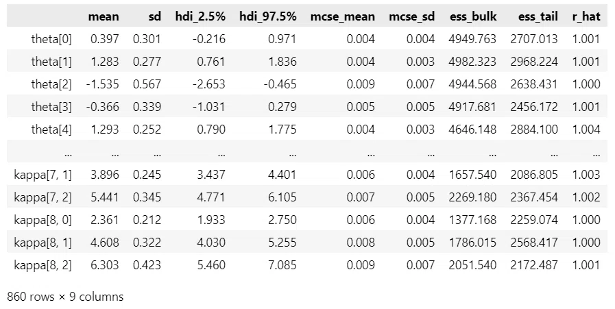
We will roughly check the summary statistics and trace plots of the posterior distribution sampling data.
### 推論データの要約統計情報の表示
pm.summary(idata_phq9, hdi_prob=0.95, round_to=3)
[Execution Result]
We will check the state of the posterior distribution sampling data using trace plots.
Only a subset of parameters is displayed.
### トレースプロットの表示
pm.plot_trace(idata_phq9, compact=False)
plt.tight_layout();
[Execution Results]
From the graph on the left, it can be seen that the four Markov chains have almost the same distribution.
In the graph on the right, the lines are drawn evenly.
It appears to have converged.

(5) Saving inference data
Let's save the inference data to a file in case we (might) need to reuse it.
We will save idata_phq9 using pickle.
### idataの保存 pickle
file = r'idata_phq9_ch17.pkl'
with open(file, 'wb') as f:
    pickle.dump(idata_phq9, f)
The code for loading it is as follows.
### idataの読み込み pickle
file = r'idata_phq9_ch17.pkl'
with open(file, 'rb') as f:
    idata_phq9_load = pickle.load(f)
Bayesian Analysis
1. Item Response Category Characteristic Curves
Bayesian analysis in the text begins by drawing item response category characteristic curves for each scale and item based on the obtained parameters, and examining the characteristics of each item.
We define the functions to calculate and plot the item response category characteristic curves.
For the calculation function, I have cited the logic from the R script in the text.
### 項目反応カテゴリ特性曲線の算出関数の定義 ※テキストのRスクリプトを引用
def calc_crf(alpha, kappa):
    x = np.arange(-3, 3.1, 0.1)
    ruiseki1 = (1 / (1 + np.exp(-1 * alpha.reshape(-1, 1) * x
                + kappa[:, 0].reshape(-1, 1)))) # カテゴリ2以上に反応する確率
    ruiseki2 = (1 / (1 + np.exp(-1 * alpha.reshape(-1, 1) * x
                + kappa[:, 1].reshape(-1, 1)))) # カテゴリ3以上に反応する確率
    ruiseki3 = (1 / (1 + np.exp(-1 * alpha.reshape(-1, 1) * x
                + kappa[:, 2].reshape(-1, 1)))) # カテゴリ4以上に反応する確率
    crf1 = 1 - ruiseki1                         # カテゴリ1に反応する確率
    crf2 = ruiseki1 - ruiseki2                  # カテゴリ2に反応する確率
    crf3 = ruiseki2 - ruiseki3                  # カテゴリ3に反応する確率
    crf4 = ruiseki3 - 0                         # カテゴリ4に反応する確率
    result = np.stack((crf1, crf2, crf3, crf4))
    return result                               # shape=(4, 20, 1000)
### 項目反応カテゴリ特性曲線の描画関数の定義
def plot_crf(crf, title): # crf.shape=(4, 20, 1000)
# x軸の値の作成
x = np.arange(-3, 3.1, 0.1)
# 描画領域の設定
fig = plt.figure(figsize=(15, 18))
# 項目ごとにaxes描画を繰り返し処理(i=項目index)
for i in range(crf.shape[1]):
# axesの作成
ax = plt.subplot(6, 4, i+1)
# カテゴリごとにaxes描画を繰り返し処理(j=カテゴリindex)
for j in range(crf.shape[0]):
ax.plot(x, crf[j, i, :], label=f'カテゴリ{j+1}')
# 修飾
ax.set(title=f'項目{i+1}', xlabel='抑うつ度 $\\theta$', ylabel='確率',
ylim=(-0.1, 1.1), yticks=(0, 0.2, 0.4, 0.6, 0.8, 1.0))
ax.grid(lw=0.3)
# 凡例の取得
if i==0:
handles, labels = ax.get_legend_handles_labels()
# 全体修飾
plt.suptitle(f'{title} の項目反応カテゴリ特性曲線', y=1.02, fontsize=16)
fig.legend(handles=handles, labels=labels,
loc='upper center', bbox_to_anchor=(0.5, 1.0), ncol=4)
plt.tight_layout()
plt.show();We plot the item response category characteristic curves for the four scales.
The text checks for any heterogeneous categories among the four category-specific curves drawn.
I believe the plotted curves generally align with the heterogeneity check in the text (since there are no figures in the text, I am unable to confirm if they are correct).
(1) SDS
### SDSの項目反応カテゴリ特性曲線の描画
# パラメータalpha, kappaのサンプルデータの平均値を算出
alpha_mean_sds = (idata_sds.posterior.alpha.stack(sample=('chain', 'draw'))
                  .mean(axis=1).data)
kappa_mean_sds = (idata_sds.posterior.kappa.stack(sample=('chain', 'draw'))
                  .mean(axis=2).data)
# 項目反応カテゴリ特性曲線の算出
crf_sds = calc_crf(alpha_mean_sds, kappa_mean_sds)
# 項目反応カテゴリ特性曲線の描画
plot_crf(crf_sds, 'SDS')
[Execution Results]

(2) CES-D
### CESDの項目反応カテゴリ特性曲線の描画
# パラメータalpha, kappaのサンプルデータの平均値を算出
alpha_mean_cesd = (idata_cesd.posterior.alpha.stack(sample=('chain', 'draw'))
                   .mean(axis=1).data)
kappa_mean_cesd = (idata_cesd.posterior.kappa.stack(sample=('chain', 'draw'))
                   .mean(axis=2).data)
# 項目反応カテゴリ特性曲線の算出
crf_cesd = calc_crf(alpha_mean_cesd, kappa_mean_cesd)
# 項目反応カテゴリ特性曲線の描画
plot_crf(crf_cesd, 'CES-D')
[Execution Results]

(3) BDI-II
### BDIの項目反応カテゴリ特性曲線の描画
# パラメータalpha, kappaのサンプルデータの平均値を算出
alpha_mean_bdi = (idata_bdi.posterior.alpha.stack(sample=('chain', 'draw'))
                   .mean(axis=1).data)
kappa_mean_bdi = (idata_bdi.posterior.kappa.stack(sample=('chain', 'draw'))
                   .mean(axis=2).data)
# 項目反応カテゴリ特性曲線の算出
crf_bdi = calc_crf(alpha_mean_bdi, kappa_mean_bdi)
# 項目反応カテゴリ特性曲線の描画
plot_crf(crf_bdi, 'BDI-II')
[Execution Results]

(4) PHQ-9
### PHQ9の項目反応カテゴリ特性曲線の描画
# パラメータalpha, kappaのサンプルデータの平均値を算出
alpha_mean_phq9 = (idata_phq9.posterior.alpha.stack(sample=('chain', 'draw'))
                   .mean(axis=1).data)
kappa_mean_phq9 = (idata_phq9.posterior.kappa.stack(sample=('chain', 'draw'))
                   .mean(axis=2).data)
# 項目反応カテゴリ特性曲線の算出
crf_phq9 = calc_crf(alpha_mean_phq9, kappa_mean_phq9)
# 項目反応カテゴリ特性曲線の描画
plot_crf(crf_phq9, 'PHQ-9')
[Execution Results]


2. Test Information Curve (TIC)
Test Information (TI) is said to be an indicator representing the estimation accuracy of depression levels.
This corresponds to Figure 17.1 in the text.
We define the function to calculate item information.
For this, I have cited the logic from the R script in the text.
### 項目情報量IIFの算出関数の定義 ※テキストのRスクリプトを引用
def calc_iif(alpha, kappa):

    # alphaの形状を(n, 1)に変換
    alpha = alpha.copy().reshape(-1, 1)

    # x軸の値の設定
    x = np.arange(-3, 3.1, 0.1)

    # カテゴリn以上に反応する確率の算出 n=(1, 2, 3, 4, 5)
    ruiseki1 = np.ones(len(x))                  # カテゴリ1以上に反応する確率=1
    ruiseki2 = (1 / (1 + np.exp(-1 * alpha * x + kappa[:, 0].reshape(-1, 1))))
    ruiseki3 = (1 / (1 + np.exp(-1 * alpha * x + kappa[:, 1].reshape(-1, 1))))
    ruiseki4 = (1 / (1 + np.exp(-1 * alpha * x + kappa[:, 2].reshape(-1, 1))))
    ruiseki5 = np.zeros(len(x))                 # カテゴリ5以上に反応する確率=0

    # カテゴリnに反応する確率の算出 n=(1, 2, 3, 4)
    CRF1 = ruiseki1 - ruiseki2                  # カテゴリ0に反応する確率
    CRF2 = ruiseki2 - ruiseki3                  # カテゴリ1に反応する確率
    CRF3 = ruiseki3 - ruiseki4                  # カテゴリ2に反応する確率
    CRF4 = ruiseki4 - ruiseki5                  # カテゴリ3に反応する確率

    # カテゴリnに反応する確率の微分 n=(1, 2, 3, 4)
    bibun1 = alpha * (ruiseki1 * (1 - ruiseki1) - ruiseki2 * (1 - ruiseki2))
    bibun2 = alpha * (ruiseki2 * (1 - ruiseki2) - ruiseki3 * (1 - ruiseki3))
    bibun3 = alpha * (ruiseki3 * (1 - ruiseki3) - ruiseki4 * (1 - ruiseki4))
    bibun4 = alpha * (ruiseki4 * (1 - ruiseki4) - ruiseki5 * (1 - ruiseki5))

    # カテゴリnのカテゴリ情報量の算出 n=(1, 2, 3, 4)
    CIF1 = bibun1**2 / CRF1                     # カテゴリ0のカテゴリ情報量
    CIF2 = bibun2**2 / CRF2                     # カテゴリ1のカテゴリ情報量
    CIF3 = bibun3**2 / CRF3                     # カテゴリ2のカテゴリ情報量
    CIF4 = bibun4**2 / CRF4                     # カテゴリ3のカテゴリ情報量

    # 項目情報量の算出
    IIF = CIF1 + CIF2 + CIF3 + CIF4

    return IIF
We calculate the test information for the four scales.
### テスト情報量TIFの算出
tif_phq9 = calc_iif(alpha_mean_phq9, kappa_mean_phq9).sum(axis=0)
tif_bdi = calc_iif(alpha_mean_bdi, kappa_mean_bdi).sum(axis=0)
tif_cesd = calc_iif(alpha_mean_cesd, kappa_mean_cesd).sum(axis=0)
tif_sds = calc_iif(alpha_mean_sds, kappa_mean_sds).sum(axis=0)
[Execution Results] None
We plot them.
### テスト情報量の描画 ★図17.1に相当

# x軸の値の設定
xval = np.arange(-3, 3.1, 0.1)
# 描画領域の設定
fig, ax = plt.subplots(figsize=(6, 5))
# PHQ-9のテスト情報量曲線の描画
ax.plot(xval, tif_phq9, ls='-', label='PHQ-9')
# BDI-IIのテスト情報量曲線の描画
ax.plot(xval, tif_bdi, ls='--', label='BDI-II')
# CES-Dのテスト情報量曲線の描画
ax.plot(xval, tif_cesd, ls=':', lw=2, label='CES-D')
# SDSのテスト情報量曲線の描画
ax.plot(xval, tif_sds, ls='-.', label='SDS')
# 修飾
ax.set(xlabel='抑うつ度 $\\theta$', ylabel='テスト情報量 $TI$',
       title='テスト情報量曲線')
plt.legend()
plt.grid(lw=0.5);
[Execution Results]
It is said that the Test Information Function (TIF) allows us to examine which scale is suitable for estimating the depression level of respondents with high (or low) levels of depression.
As the text suggests, CES-D, BDI-II, and PHQ-9 show similar trends, and it is thought that the estimation accuracy for people with relatively high levels of depression will be higher.
It is thought that SDS will have higher estimation accuracy for people with relatively low levels of depression.


3. Relative Efficiency Curve (REC)
The relative curve RE is the ratio of the TI of two scales.
By utilizing the relative efficiency curve, it is said that it becomes possible to compare measurement efficiency between scales at core levels of depression.
This corresponds to Figures 17.2 and 17.3 in the text.
Calculate the relative efficiency RE of the four scales.
### 相対効率REの算出
bdi_vs_phq9 = tif_bdi / tif_phq9
cesd_vs_phq9 = tif_cesd / tif_phq9
sds_vs_phq9 = tif_sds / tif_phq9
cesd_vs_bdi = tif_cesd / tif_bdi
sds_vs_bdi = tif_sds / tif_bdi
sds_vs_cesd = tif_sds / tif_cesd
[Execution Results] None
Plot the REC between CES-D, BDI-II, and PHQ-9.
### CES-D, BDI-II, PHQ-9の相対効率曲線の描画 ★図17.2に相当

# x軸の値の設定
xval = np.arange(-3, 3.1, 0.1)
# 描画領域の設定
fig, ax = plt.subplots(figsize=(6, 5))
# bdi/phq9の相対効率曲線の描画
ax.plot(xval, bdi_vs_phq9, ls='-', label='BDI-II / PHQ-9')
# cesd/phq9の相対効率曲線の描画
ax.plot(xval, cesd_vs_phq9, ls='-.', label='CES-D / PHQ-9')
# cesd/bdiのテスト情報量曲線の描画
ax.plot(xval, cesd_vs_bdi, ls='--', label='CES-D / BDI-II')
# 修飾
ax.set(xlabel='抑うつ度 $\\theta$', ylabel='相対効率 $RE$',
       title='CES-D, BDI-II, PHQ-9間の相対効率曲線')
plt.legend()
plt.grid(lw=0.5);
[Execution Results]
In the comparison of BDI-II / PHQ-9, it is interpreted that BDI-II has higher measurement efficiency when the relative efficiency RE on the vertical axis is greater than the ratio of the number of items, 21 / 9 = 2.33, at depression levels (θi ≤ 2.97, 2.47 ≤ θi).

Plot the REC between SDS and the other scales.
### SDSとCES-D, BDI-II, PHQ-9の相対効率曲線の描画 ★図17.3に相当

# x軸の値の設定
xval = np.arange(-3, 3.1, 0.1)
# 描画領域の設定
fig, ax = plt.subplots(figsize=(6, 5))
# sds/phq9の相対効率曲線の描画
ax.plot(xval, sds_vs_phq9, ls=':', lw=2, label='SDS / PHQ-9')
# sds/bdiの相対効率曲線の描画
ax.plot(xval, sds_vs_bdi, ls='-', label='SDS / BDI-II')
# sds/cesdのテスト情報量曲線の描画
ax.plot(xval, sds_vs_cesd, ls=(0, (3, 1, 1, 1)), label='SDS / CES-D')
# 修飾
ax.set(xlabel='抑うつ度 $\\theta$', ylabel='相対効率 $RE$',
       title='SDSとCES-D,BDI-II,PHQ-9間の相対効率曲線')
plt.legend()
plt.grid(lw=0.5);
[Execution Results]


4. Conversion Table Between Scale Scores
Create a 'conversion table' that calculates the expected values of the scale scores for the four scales within the range of depression level θi from -3 to 3.
This is Table 17.1 in the text.
### 尺度得点間の換算表の作成 ★表17.1に相当

# θの値の設定
theta_val = np.arange(-3, 3.1, 0.1).round(1)

# 尺度得点の期待値とTCFの算出 ★テキストのRスクリプトに準拠
expected_phq9 = np.array([
    (np.arange(0, 4).reshape(-1, 1) * crf_phq9[:, i, :]).sum(axis=0)
    for i in range(9)])
tcf_phq9 = expected_phq9.sum(axis=0)
expected_bdi = np.array([
    (np.arange(0, 4).reshape(-1, 1) * crf_bdi[:, i, :]).sum(axis=0)
    for i in range(21)])
tcf_bdi = expected_bdi.sum(axis=0)
expected_cesd = np.array([
    (np.arange(0, 4).reshape(-1, 1) * crf_cesd[:, i, :]).sum(axis=0)
    for i in range(20)])
tcf_cesd = expected_cesd.sum(axis=0)
expected_sds = np.array([(
    np.arange(1, 5).reshape(-1, 1) * crf_sds[:, i, :]).sum(axis=0)
    for i in range(20)])
tcf_sds = expected_sds.sum(axis=0)

# データフレーム化
tcf_df = pd.DataFrame({'θ': theta_val,
                       'SDS': tcf_sds,
                       'CES-D': tcf_cesd,
                       'BDI-II': tcf_bdi,
                       'PHQ-9': tcf_phq9,
                      }).set_index('θ', drop=True)

# データフレームの表示
pd.set_option('display.max_rows', 100)
display(tcf_df.round(2))
[Execution Results]
The values generally match those in the conversion table in the text.


Let's visualize the conversion table.
### テスト特性曲線の描画
tcf_df.plot(kind='line', figsize=(6, 5), xlabel='抑うつ度 $\\theta$',
            ylabel='尺度得点の期待値', title='テスト特性曲線')
plt.grid(lw=0.5)
[Execution Results]

This concludes Chapter 17.
Conclusion
Item Response Theory
By practicing with the 'Fun Bayesian Modeling' book series, I have had many opportunities to encounter Bayesian models for Item Response Theory.
In addition to the latent variable θ representing the trait value, and the item discrimination α and difficulty β, there is also κ, which appeared this time.
It is thrilling to see latent variables emerge from response values (actual values), and I was able to work on this very enjoyably.
I am also attracted to the beauty of the curves in the Item Characteristic Curves, which plot response probabilities corresponding to the magnitude of the trait value θ.
While it may not be a method used on a daily basis, it is a method I would like to remember from time to time.

The End
Series Articles
Next Article
Previous Article
Table of Contents
Blog Introduction
I am writing seven series of articles on note.
Please come and take a look!
1. Relaxed Statistics
This is a blog that roughly explores probability and statistics using the Statistical Test Grade 2 problem collection as a guide.
Feel free to read it as if it were casual conversation. Please come and take a look.
It corresponds to the Statistical Test Grade 2 Official Problem Collection CBT Edition.
Sample code for Python and EXCEL is also available.
2. Experiment! Fun Bayesian Modeling 1 & 2 with PyMC Ver. 5
I will draw and analyze the Bayesian models used in psychological research from the books 'Fun Bayesian Modeling' and 'Fun Bayesian Modeling 2' using PyMC Ver. 5.
Like this book, many Bayesian models are written in R + Stan.
I strive to explore the possibilities of PyMC and make Bayesian modeling easy to practice.
Since these are familiar and easy-to-visualize themes, please try running them with PyMC and let's enjoy it together!
3. Experiment! Iwanami Data Science 1 Bayesian Modeling with PyMC Ver. 5
I will draw and analyze the Bayesian models by four Bayesians from the book 'Experiment! Iwanami Data Science Vol. 1' using PyMC Ver. 5.
This book is a great resource for learning the basics of Bayesian programming.
I feel like I've become friends with Bayesian methods by happily running PyMC models.
Everyone, please try running them with PyMC, and let's play and learn together!
4. Fun Transcription: Bayesian, Python, etc.
I will blog about the results of my 'book transcription activities' for Bayesian, Python, and others.
I am mainly working on translations into Python.
I hope this will serve as sample code for fellow learners who are also transcribing. 🍀
5. Introduction to Time Series Analysis for Psychology starting with R and Stan, using Python and PyMC Ver. 5
I will practice the time series analysis from the book 'Introduction to Time Series Analysis for Psychology starting with R and Stan' using Python and PyMC Ver. 5.
This book is packed with time series analysis themes!
I realized the depth of time series analysis.
I will enjoy learning time series analysis with my favorite language, Python.
6. Writing about Data Science-like things
I write columns on statistics, data analysis, AI, machine learning, and Python on an irregular basis.
There are many articles related to statistics and data science books.
Series on 'Statistics', 'Python', 'Math and Python', and 'R' have been created.
7. Python Machine Learning Programming Practice Journal
I wrote an article about my various thoughts when studying the book 'Python Machine Learning: PyTorch & scikit-learn Edition'.
This book is a textbook for scikit-learn and PyTorch.
Please feel free to give it a try.
Thank you very much for reading until the end.
いいなと思ったら応援しよう!
 応援ありがとうございます。これからもがんばって記事を作成します!