SYSTEM NOTICE

Auto translation by AI. Be sure, accuracy, nuances and authorial intent may not be fully reflected.

Bayesian Modeling for Chapter 8, "'Stories' Challenged by Statistical Modeling," using PyMC Ver. 5

2024年3月23日 11:01

This article is a statistical documentary depicting the process of "experimentally" implementing the Bayesian models from Chapter 8, "'Stories' Challenged by Statistical Modeling," in the text "Fun Bayesian Modeling 2" using PyMC Ver. 5.

In this chapter, we predict the reactions of viewers of the popular animated work "Violet Evergarden" using Bayesian modeling.
From the beginning, where three mathematical models are constructed according to the work's structure, to the end, where a negative binomial distribution is modeled, it is a brilliant piece of storytelling that captivates the reader.
Please be sure to read the text!

Illustration of students reading a textbook together: from "Irasutoya"

Well then, let's enjoy the world of PyMC Bayesian modeling!

Please refer to the article at this link for the introduction to the text, citation format, series preface, and version information for PyMC, etc.

The data used in the text, along with sample scripts for R, Stan, etc., can be downloaded from the publisher's website.

Summary

Overview of the text

Author: Dr. Jiro Sakamoto
Model Difficulty: ★★★★・ (Somewhat difficult)

Self-evaluation

Rating

$$
\begin{array}{c:c:c}
Implementation Accuracy & ★★★★★ & GoooD! \\
Result Reproducibility & ★★★★★ & Best✨ \\
Fun & ★★★★★ & Fun! \\
\end{array}
$$

Illustration of a flower-shaped evaluation stamp: from "Irasutoya"

Evaluation Points

For the first time in a while, the results almost perfectly matched the text! I'm so happy!!!

Ingenuity, Joy, and Reflections

I learned that "mean" and "dispersion" can be used as parameters for the negative binomial distribution. It's like the normal distribution! In the future, when considering probability distributions for discrete values (count data), I want to check the dispersion of observed values and use the Poisson distribution and negative binomial distribution appropriately!
When incorporating the three mathematical models into a Bayesian model, it is necessary to code the selection and conditional branching of the mathematical models. Regarding the conditional branching code, I was able to convert it to PyMC5 by referring to the following article. Thank you very much!

Illustration of people gathering (children): from "Irasutoya"

Model Overview

Overview of the text's research and experiments

■ Introduction to the work
This chapter focuses on the TV animation series "Violet Evergarden."
I looked up an overview of this work on Wikipedia.

A total of 13 episodes aired from January 11, 2018, to April 5, 2018
The original work is the novel "Violet Evergarden" by Kana Akatsuki
Two theatrical versions have been adapted into films

As I read through the information from the web search, I realized that this is a work loved by many viewers.

Illustration of a person crying while watching TV (female): From "Irasutoya"

■ Overview of the data
The text uses data obtained from the "ShangriLa Anime API Server" provided by the Akihabara IT Strategy Research Institute.
In this article, I will also borrow data sourced from the Akihabara IT Strategy Research Institute.
Thank you very much!

I will borrow and include the brief history of the data from the text.
Note that the one-day discrepancy with the Wikipedia dates is likely because the text uses the previous day's date for broadcast slots after 24:00 (midnight).

The data is the "number of new followers on the official Twitter account of the work during the period from the first broadcast date of January 10, 2018, to six days after the final episode broadcast date: April 10", which is the "increase in followers of the official work Twitter account".
The data for the week of March 28, the broadcast date of episode 12, and April 4, the final episode broadcast date, is missing.

In summary, it is time-series data of follower increases that "contains missing values."

Illustration of an influencer (male): From "Irasutoya"

■ Challenges addressed in this chapter
The author states, "The specific challenge of this chapter is to quantitatively model the (work's) structure and predict the actual social response to the work."
A three-part structure consisting of 'Jo-Ha-Kyu' (introduction, development, and conclusion) is assumed for the work's structure.
The beginning 'Jo' (introduction), the development 'Ha' (break), and the 'Kyu' (rapid) that builds up to the climax.
The text constructs a mathematical model by mapping the work's structure to the number of follower increases.
It seems there is an awareness of the issue that the impact of the work influences the number of Twitter follower increases.

■ Mathematical model
I will borrow Figure 8.2 from the text to share the image of the mathematical model according to the development of the work.

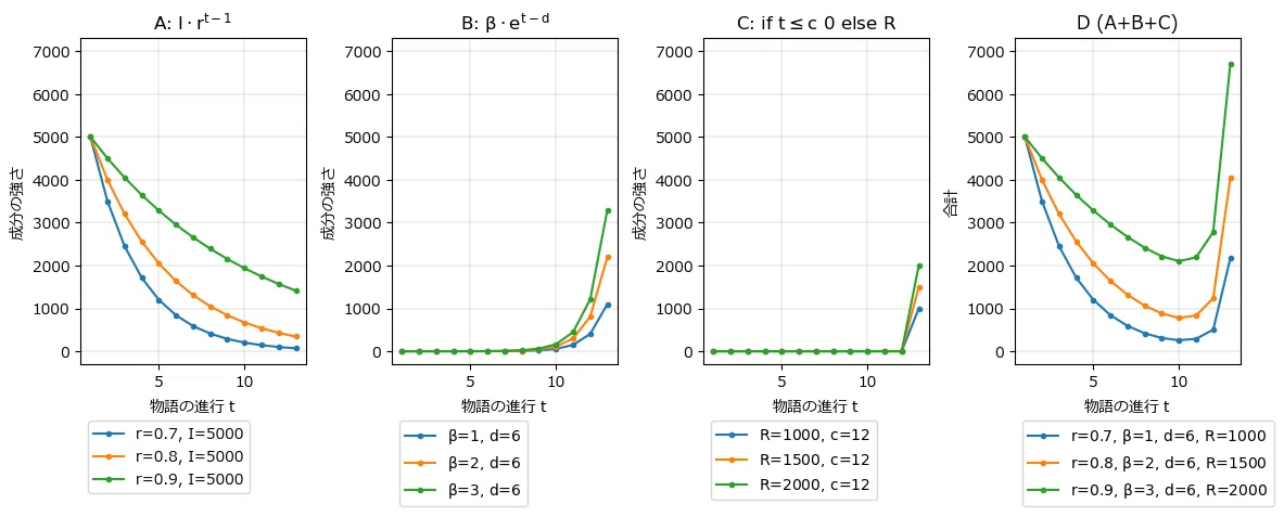
From the left, component A for 'Jo', component B for 'Ha', component C for 'Kyu', and D, which is the sum of all components.
The horizontal axis of the graph is the episode number of the work (progression of the story/passage of time), and the vertical axis is the strength of the component indicating the impact of the work.
Also, the mathematical model for each component is appended to the graph title.

Component A of the beginning 'Jo' is a curve that starts with a strong impact and gradually settles down.
Component B of 'Ha' is a curve that shows a gradual rise from the second half.
The final 'Kyu' is a curve related to the climax shown in the final episode.
Looking at D, which is the sum of the three curves, one can clearly see the initial excitement, the settling down in the middle, and the great excitement at the end.

Illustration of a mathematician (female): From "Irasutoya"

Here are the mathematical expressions for each component. I will borrow them from the text.

The main component of the introduction, $${A_t}$$, is expressed for each episode $${t,\ t=1, \cdots, 13}$$ of the 13 episodes as an exponential function $${{\gamma^{t-1}}}$$ using the introduction impact $${I}$$ and the impact decay trend parameter $${\gamma}$$ ($${0 \leq \gamma \leq 1}$$).

$$
A_t = I \cdot \gamma^{t-1}
$$

Quoted from the text

Since $${\gamma}$$ is a positive decimal between 0 and 1, as the episode number progresses, the value of $${t-1}$$ increases, and the value of $${\gamma^{t-1}}$$ decreases.

◆◆◆

The main component of the development (Ha), $${B_t}$$, is expressed for each episode $${t, \ t=1, \cdots, 13}$$ out of the total 13 episodes using an exponential function $${\exp(t-d)}$$, which utilizes the degree of rise in the latter half's upward trend, $${\beta}$$, and $${d}$$ ($${0 < d < 13}$$), which adjusts the turning point where it shifts to an upward trend.

$$
B_t = \beta \cdot \exp(t-d)
$$

Quoted with partial modifications to the mathematical formulas in the text

$${\exp(t-d)}$$ refers to the base of the natural logarithm $${e}$$ raised to the power of $${t-d}$$.
When the episode number $${t}$$ is smaller than $${d}$$, that is, before it turns to an upward trend, $${t-d}$$ is a negative value, so $${\exp(t-d)}$$ is a small value.
On the other hand, once it passes the episode number $${d}$$ where it turns to an upward trend, $${t-d}$$ becomes a positive value, so $${\exp(t-d)}$$ becomes a large value, indicating a rise.

◆◆◆

The main component of the conclusion (Kyu), $${C_t}$$, is expressed by a conditional expression that provides the impact parameter $${R}$$ ($${R > 0}$$) of the climax only after the timing $${c}$$ when it switches to the climax.

$$
\begin{matrix}
C_t = 0 & (\text{if} \quad t \leq c) \\
C_t = R & (\text{if} \quad t > c) \\
\end{matrix}
$$

Quoted from the text

Assuming the timing $${c}$$ to switch to the climax is episode 12, $${C_t}$$ is 0 until episode 12, meaning there is no climax impact.
When it reaches episode 13, the climax impact $${R}$$ hits hard!

These mathematical models are incorporated into a Bayesian model that "analyzes the relationship between the dramatic development of Violet Evergarden and fan reactions"!
A Bayesian model plus a mathematical model—something amazing seems about to happen.

Illustration of a transforming robot: from "Irasutoya"

Before modeling: Negative Binomial Distribution

The text proceeds to even more impactful modeling.
That is, assuming a "negative binomial distribution" for the probability distribution followed by the objective variable, the "number of follower increases $${Y_t}$$"!assuming a "negative binomial distribution"!

■ Negative Binomial Distribution
The negative binomial distribution is a discrete probability distribution.
It seems there are the following two definitions.

When repeating independent trials with a success probability $${p}$$, the distribution followed by the number of trials $${y}$$ until $${r}$$ successes occur
When repeating independent trials with a success probability $${p}$$, the distribution followed by the number of failures $${y}$$ until $${r}$$ successes occur

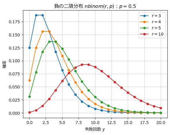
I will post an image of the probability mass function of the negative binomial distribution from Definition 2.
I used scipy.stats' nbinom.

■ Another aspect of the negative binomial distribution
However, the text teaches us another aspect of the negative binomial distribution.
That is, "The negative binomial distribution is a probability distribution with two parameters: mean $$\boldsymbol{\mu}$$ and dispersion $$\boldsymbol{\varphi}$$" (Definition 3).

Based on Definition 2. (where $${y}$$ is the number of failures), calculating the success probability $${p}$$ and the number of successes $${r}$$ using the mean $$\mu$$ and dispersion $$\varphi$$ results in the following equations.

$$
\begin{align*}
r &= \varphi \\
p &= \cfrac{\varphi}{\mu + \varphi} \\
\end{align*}
$$

Cited from information on the following website

This formula was cited from the information on page 11 of the following website.
Thank you!

Let's plot the probability mass function of the negative binomial distribution with Definition 3. (mean $$\mu$$, dispersion $$\varphi$$).

As the value of the dispersion $$\varphi$$ increases, a peak is formed, and the sharpness of the peak increases.
An increase in the sharpness of the peak means that the dispersion decreases.
In other words, as the value of $$\varphi$$ increases, the dispersion decreases.

■ Negative binomial distribution and Poisson distribution
The curve in the figure above resembles the probability mass function of a Poisson distribution.
The text gently taught me that we use the negative binomial distribution for modeling when it cannot be expressed by a Poisson distribution.

In the context of statistical modeling, the negative binomial distribution is often used to deal with overdispersion in the Poisson distribution. That is, the negative binomial distribution is sometimes applied when it is judged that the variation in the observed data is larger (overdispersion) than predicted by the Poisson distribution, which has the constraint that the mean and variance are equal.

Cited from the text; I added the bold text

The dispersion parameter $$\varphi$$ really plays a key role!
It is said that when $$\varphi=\infty$$, it matches the Poisson distribution.
Please check the derivation of the relationship between the negative binomial distribution and the Poisson distribution in the text!

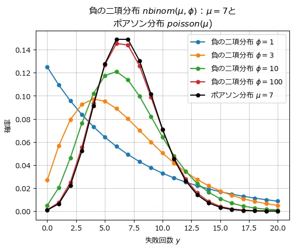
Let's plot the probability mass function of the negative binomial distribution in contrast to the Poisson distribution.

As the value of $$\varphi$$ increases, the negative binomial distribution approaches the Poisson distribution.
When $$\varphi=\infty$$, the negative binomial distribution and the Poisson distribution match.

■ Personal excitement✨
Having mean and dispersion as parameters means...
the negative binomial distribution can be used like a normal distribution for discrete variables and count data.
In the future, when doing Bayesian modeling of count data, I would like to utilize the negative binomial distribution in addition to the Poisson distribution!

Standing ovation illustration: from "Irasutoya"

The introduction has become long...

Modeling in the text

■ Modeling, negative binomial distribution, and mathematical models
The text states that "the number of follower increases $${Y_i}$$ follows a negative binomial distribution with mean $$\mu$$ and dispersion $$\varphi$$".
And the sum of the three components mentioned above, $${A_t+B_t+C_t}$$, is used for the mean $$\mu$$.
A rendezvous between the negative binomial distribution and mathematical models✨

■ Objective variable and parameters of interest
The objective variable is the number of follower increases $${Y_{it}}$$.
The subscript $${t}$$ represents the broadcast episodes of all 13 episodes ($${t=1, \cdots, 13}$$).
The subscript $${i}$$ is the number of days elapsed within the week from the broadcast date for each broadcast episode $${t}$$ ($${i=1, \cdots, 7}$$).
It seems that no particular parameters of interest have been set.
I am focusing on the predicted values of the objective variable $${Y}$$ calculated and sampled by MCMC.

■ Model Equations
First, I will write out the equations as they appear in the text.

$$
\begin{align*}
Y_{it} &\sim \text{NegativeBinomial}\ (\mu_{it},\ \varphi) \\
\mu_{it} =
\begin{cases}
\mu_t & i=1 \\
\mu_t \cdot w \cdot k^{i-2} & i=2, \cdots, 7 \\
\end{cases} \\
\mu_{t} &= A_t + B_t + C_t \\
A_t &= I \cdot \gamma^{t-1} \\
B_t &= \beta \cdot \exp(t-d) \\
C_t =
\begin{cases}
0 &\text{if}\ & t \leq c \\
R &\text{if}\ & t > c \\
\end{cases} \\
\end{align*}
$$

Quoted from the text

■ Supplementary notes on parameters
${w}$ (${1 < w}$) is the "carry-over effect to the next day" coefficient, which is multiplied by the estimated follower increase ${\mu_t}$ on the broadcast day.
Since the broadcast time was late at night on a weekday, this accounts for viewers who record the show and watch it the following day.
${k}$ (${0 \leq k \leq 1}$) is the decay coefficient for the intra-week downward trend in follower increases.
This accounts for the downward trend in follower increases during the week from the day after the broadcast until the next broadcast day.

■ Supplementary notes on prior distributions of parameters
For the prior distributions of the parameters, we assume uniform distributions.
The range of the uniform distribution is not explicitly stated in the text.
The initial impact ${I}$ is taken as the number of followers on the first broadcast day ${y_{t=1}}$.
The parameter ${R}$ for component ${C_t}$ is set to a sufficiently large upper bound (${0 < R < 10000}$), assuming it is added to the final episode.

■ Analysis and Analysis Results
I believe the descriptions of the analysis methods and numerical values in the text are accurate, so I recommend reading the text.
Please refer to the "PyMC Implementation" chapter for analysis using inferred values from my own PyMC model.

ON AIR lamp illustration: From "Irasutoya"

PyMC Implementation

Let's enjoy PyMC & Python !

Preparation and Data Verification

1. Imports

### インポート

# ユーティリティ
import pickle

# 数値・確率計算
import pandas as pd
import numpy as np
import scipy.stats as stats

# PyMC
import pymc as pm
import pytensor.tensor as pt
import arviz as az

# 描画
import matplotlib.pyplot as plt
plt.rcParams['font.family'] = 'Meiryo'

# ワーニング表示の抑制
import warnings
warnings.simplefilter('ignore')

2. Plots used for modeling explanation
I will post four pieces of code to draw the figures used in the "Model Overview" chapter.

① Example of story development composition using a mathematical model
This corresponds to Figure 8.2 in the text.

### 数理モデルによるストーリー展開の構成例 ※図8.2に相当

### 設定
## データ設定：t＝1～13
t = np.arange(1, 14)
## 描画設定
label = ['物語の進行 $t$', '成分の強さ', '合計']
title = ['A: $I \cdot r^{t-1}$', 'B: $\\beta \cdot e^{t-d}$',
         'C: $if\ t \leq c\ 0\ else\ R$', 'D (A+B+C)']
ylim = (-300, 7300)
bbox = (0, -0.15)
loc = 'upper left'

### 描画
fig, (ax1, ax2, ax3, ax4) = plt.subplots(1, 4, figsize=(12, 5))

## Aの描画
# パラメータ設定
I = 5000
rs = np.array([0.7, 0.8, 0.9])
At = np.zeros((len(rs), len(t)))
# パラメータrごとに折れ線グラフを描画
for i, r in enumerate(rs):
    # 数理モデルAt
    At[i] = I * r**(t-1)
    # 折れ線グラフの描画
    ax1.plot(t, At[i], '.-', label=f'r={r}, I={I}')
    # 修飾
    ax1.set(xlabel=label[0], ylabel=label[1], title=title[0], ylim=ylim)
    ax1.legend(bbox_to_anchor=bbox, loc=loc)
    ax1.grid(lw=0.3)

## Bの描画
# パラメータの設定
betas = np.array([1, 2, 3])
d = 6
Bt = np.zeros((len(betas), len(t)))
# パラメータβごとに折れ線グラフを描画
for i, beta in enumerate(betas):
    # 数理モデルBt
    Bt[i] = beta * np.exp(t-d)
    # 折れ線グラフの描画
    ax2.plot(t, Bt[i], '.-', label=f'$\\beta$={beta}, d={d}')
    # 修飾
    ax2.set(xlabel=label[0], ylabel=label[1], title=title[1], ylim=ylim)
    ax2.legend(bbox_to_anchor=bbox, loc=loc)
    ax2.grid(lw=0.3)

## Cの描画
# パラメータの設定
Rs = np.array([1000, 1500, 2000])
c = 12
Ct = np.zeros((len(Rs), len(t)))
# パラメータRごとに折れ線グラフを描画
for i, R in enumerate(Rs):
    # 数理モデルCt
    Ct[i] = [R if time > c else 0 for time in t]
    # 折れ線グラフの描画
    ax3.plot(t, Ct[i], '.-', label=f'$R$={R}, c={c}')
    # 修飾
    ax3.set(xlabel=label[0], ylabel=label[1], title=title[2], ylim=ylim)
    ax3.legend(bbox_to_anchor=bbox, loc=loc)
    ax3.grid(lw=0.3)

## D=A+B+Cの描画
# ３つのパラメータケースごとに折れ線グラフを描画
for i in range(3):
    # At+Bt+Ctを計算して折れ線グラフを描画
    ax4.plot(t, At[i] + Bt[i] + Ct[i], '.-',
             label=f'$r$={rs[i]}, $\\beta$={betas[i]}, $d$={d}, $R$={Rs[i]}')
    # 修飾
    ax4.set(xlabel=label[0], ylabel=label[2], title=title[3], ylim=ylim)
    ax4.legend(bbox_to_anchor=bbox, loc=loc)
    ax4.grid(lw=0.3)
plt.tight_layout();

[Execution Result]

② Probability mass function of the negative binomial distribution Definition 2

### 負の二項分布の確率質量関数 定義2
yvals = range(0, 21)
rvals = [3, 4, 5, 10]
for r in rvals:
    plt.plot(yvals, stats.nbinom.pmf(k=yvals, n=r, p=0.5), '-o', ms=5,
             label=f'$r={r}$')
plt.xlabel('失敗回数 $y$')
plt.ylabel('確率')
plt.title('負の二項分布 $nbinom(r, p)$：$p=0.5$')
plt.grid(lw=0.5)
plt.legend();

[Execution Result]

③ Probability mass function of the negative binomial distribution Definition 3 NegativeBinomial(μ,φ)

### 負の二項分布の確率質量関数 定義3 NegativeBinomial(μ,φ)
# 参考サイト https://www.slideshare.net/simizu706/ss-50994149

# 負の二項分布のパラメータの設定
mu = 7                          # μ
phis = np.array([1, 3, 10])     # φ
# パラメータpとrを計算して負の二項分布の確率質量関数を描画
for phi in phis:
    r = phi                     # 成功回数r
    p = phi / (mu + phi)        # 成功確率p
    plt.plot(yvals, stats.nbinom.pmf(k=yvals, n=r, p=p), '-o', ms=5,
             label=fr'$\phi={phi}$')
# 修飾
plt.xlabel('失敗回数 $y$')
plt.ylabel('確率')
plt.title(r'負の二項分布 $nbinom(\mu, \phi)$：$\mu=7$')
plt.grid(lw=0.5)
plt.legend();

[Execution Result]

④ Probability mass function of the negative binomial distribution Definition 3 NegativeBinomial(μ,φ) and Poisson distribution

### 負の二項分布の確率質量関数 定義3 NegativeBinomial(μ,φ)とポアソン分布
# https://www.slideshare.net/simizu706/ss-50994149

# 負の二項分布のパラメータの設定
mu = 7                          # μ
phis = np.array([1, 3, 10, 100])     # φ
# パラメータpとrを計算して負の二項分布の確率質量関数を描画
for phi in phis:
    p = phi / (mu + phi)        # 成功確率p
    r = phi                     # 成功回数r
    plt.plot(yvals, stats.nbinom.pmf(k=yvals, n=r, p=p), '-o', ms=5,
             label=fr'負の二項分布 $\phi={phi}$')
# ポアソン分布の確率質量関数を描画
plt.plot(yvals, stats.poisson.pmf(k=yvals, mu=mu), '-o', ms=5,
            label=fr'ポアソン分布 $\mu={mu}$', color='black')
# 修飾
plt.xlabel('失敗回数 $y$')
plt.ylabel('確率')
plt.title(r'負の二項分布 $nbinom(\mu, \phi)$ : $\mu=7$と' + '\n'
          r'ポアソン分布 $poisson(\mu$)')
plt.grid(lw=0.5)
plt.legend();

[Execution Result]

3. Loading Data
Load the csv file into a pandas dataframe.

### データの読み込み
data_orgn = pd.read_csv('d.csv', encoding='cp932', parse_dates=['Date'])
display(data_orgn)

[Execution Result]
This is data with 92 rows.
The Follower column contains the follower count.
We will calculate the follower increase in the next preprocessing step.

4. Data Preprocessing
Use pandas' diff() to subtract the follower count from one day ago (one row ago) to generate the follower increase.
Also, for model convenience, we divide the data into two sets: "data_full" containing all dates, and "data_base" containing only broadcast dates.

### データの前処理

## data_fullの作成
# 読み込みデータのコピーを取得
data_full = data_orgn.copy()
# フォロワー増加数列の作成（1行前のフォロワー数を差し引く）、１行目を削除
data_full['Delta'] = data_full['Follower'].diff(1)
data_full = data_full.iloc[1:, :]
# 放送回（エピソード番号）列の作成：R・fullデータのEpisodeIndex
data_full['EpisodeNo'] = np.repeat(range(1, 14), 7)[:len(data_full)]
# 週番号列の作成：R・fullデータのInnerIndex
data_full['InnerNo'] = np.tile(range(1, 8), 13)[:len(data_full)][:len(data_full)]

## 放送日行のみを取り出したdata_baseの作成
data_base = data_full.query('OnAir == "放送日"').reset_index()

## 前処理後のデータ表示
display(data_full)
display(data_base)

[Execution Result]
This is data_full.
The Date column is the date, OnAirDate is the broadcast date, Delta is the follower increase, EpisodeNo is the episode number, and InnerNo is a sequential number from 1 to 7 within the week.

This is data_base. Since it is filtered only by broadcast dates, the number of data entries is 13.

5. Plotting the Time Series of Follower Increases
This corresponds to Figure 8.3 in the text.

### Twitter公式アカウントのフォロワー増加数推移の描画 ※図8.3に相当

## データの準備
# 放送日の翌日日付の算出
nextdate = data_full.query('OnAir =="放送日"')['Date'] + pd.Timedelta(days=1)

## 描画
# 描画領域の指定
plt.figure(figsize=(12, 4))
# フォロワー増加数の描画
plt.plot(data_full['Date'], data_full['Delta'], '.-', color='tab:blue',
         label='フォロワー増加数')
# 放送日のフォロワー増加数の四角点の描画
plt.scatter(data=data_full.query('OnAir =="放送日"'), x='Date', y='Delta',
            marker='s', color='tab:blue', label=None)
# 放送日付の垂直線の描画
for date in data_full.query('OnAir =="放送日"')['Date']:
    plt.axvline(date, color='gray', lw=0.5)
# 放送日の翌日日付の垂直線の描画
for date in nextdate:
    plt.axvline(date, color='black', lw=0.8, ls='--')
# 放送日・放送日翌日の凡例用のダミー描画
plt.plot([], [], color='gray', lw=0.5, ls='--', label='放送日')
plt.plot([], [], color='gray', lw=0.8, ls='--', label='放送日の翌日')
# x軸目盛ラベルに放送日の翌日日付を表示
plt.xticks(nextdate, rotation=30)
# 修飾
plt.title(f'Twitter公式アカウントのフォロワー増加数推移')
plt.xlabel('日付')
plt.ylabel('フォロワー増加数')
plt.legend(loc='upper left');

[Execution Result]
It feels similar to the shape of the mathematical model.
There is no data around March 29th due to missing values.

Model Construction

Mathematical Representation of the Model
This is a "pseudo-mathematical" notation that incorporates the feel of the PyMC model we want to aim for.

$$
\begin{align*}
\gamma &\sim \text{Uniform}\ (\text{lower}=0,\ \text{upper}=1) \\
d &\sim \text{Uniform}\ (\text{lower}=0,\ \text{upper}=13) \\
\beta &\sim \text{Uniform}\ (\text{lower}=0,\ \text{upper}=100) \\
R &\sim \text{Uniform}\ (\text{lower}=0,\ \text{upper}=10000) \\
w &\sim \text{Uniform}\ (\text{lower}=1,\ \text{upper}=10) \\
k &\sim \text{Uniform}\ (\text{lower}=0,\ \text{upper}=1) \\
k_{final} &\sim \text{Uniform}\ (\text{lower}=0,\ \text{upper}=1) \\
\varphi &\sim \text{Uniform}\ (\text{lower}=0,\ \text{upper}=10000) \\
\\
A_t &= Y_t \times \gamma^{t-1}, \quad \text{dims}=episodeNo \\
B_t &= \beta \times \exp (t-d), \quad \text{dims}=episodeNo \\
C_t &= [0,0,0,0,0,0,0,0,0,0,0,0,R]
\\
\mu_t &= A_t + B_t + C_t, \quad \text{dims}=episodeNo \\
\mu_i &= \text{calc\_mui}, \quad \text{dims}=y_idata \\
\\
Y_t likelihood &\sim \text{NegativeBinomial}\ (\text{mu}=\mu_t,\ \text{alpha}=\varphi,\ \text{dims}=episodeNo) \\
Y_i likelihood &\sim \text{NegativeBinomial}\ (\text{mu}=\mu_i,\ \text{alpha}=\varphi,\ \text{dims}=y_idata) \\
\\
Y_tpred &\sim \text{NegativeBinomial}\ (\text{mu}=\mu_t,\ \text{alpha}=\varphi,\ \text{dims}=episodeNo) \\
Y_ipred &\sim \text{NegativeBinomial}\ (\text{mu}=\mu_i,\ \text{alpha}=\varphi,\ \text{dims}=y_idata) \\
\end{align*}
$$

1. Model Definition
Define the initial values and the functions to be used within PyMC.
calc_muI() is a function that calculates the value of muI according to the conditions.

### モデル定義の準備

## 初期値設定
# 放送回（エピソード番号）のリスト化
episode_no = np.arange(1, 14)
# クライマックスタイミングc
c = 12

## muI計算関数 stanコードのmu_i[j]の計算ロジック
# 参考にした情報: https://qiita.com/Gyutan/items/691331556641ddbf88f3
def calc_muI(muT, epiNo, innerNo, c, w, k, kFinal):
    case1 = muT                                     # case1: 週の1日め
    case2 = muT * w * k**(innerNo - 2)              # case2: 0<放送回<=c
    case3 = muT * w * kFinal**(innerNo - 2)         # case3: 放送回>c
    return pt.switch(pt.eq(innerNo, 1),   case1,  
                     pt.switch(epiNo > c, case3,
                                          case2))

We describe the model faithfully to the mathematical expression.
"pt" in the formula stands for pytensor.tensor, which is used for tensor calculation processing.

### モデルの定義
with pm.Model() as model:
    
    ### データ関連定義
    # coordの定義
    model.add_coord('yiData', values=data_full.index, mutable=True)
    model.add_coord('ytData', values=data_base.index, mutable=True)
    model.add_coord('epiNo', values=episode_no, mutable=True)
    # dataの定義
    yi = data_full['Delta'].values  # 欠損値を含むためConstantDataにできない
    yt = data_base['Delta'].values  # 欠損値を含むためConstantDataにできない
    epiNo = pm.ConstantData('epiNo', value=episode_no, dims='episodeNo')
    innerNoData = pm.ConstantData('innerNoData',
                                  value=data_full['InnerNo'].values,
                                  dims='yiData')
    epiNoData = pm.ConstantData('epiNoData',
                                  value=data_full['EpisodeNo'].values,
                                  dims='yiData')
    epiNoIdx = pm.ConstantData('epiNoIdx',
                               value=data_full['EpisodeNo'].values - 1,
                                dims='yiData')

    ### 事前分布
    gamma = pm.Uniform('gamma', lower=0, upper=1)    
    d = pm.Uniform('d', lower=0, upper=13)
    beta = pm.Uniform('beta', lower=0, upper=100)
    R = pm.Uniform('R', lower=0, upper=10000)
    w = pm.Uniform('w', lower=1, upper=10)
    k = pm.Uniform('k', lower=0, upper=1)
    kFinal = pm.Uniform('kFinal', lower=0, upper=1)
    phi = pm.Uniform('phi', lower=0, upper=10000)

    ### 数理モデルの計算
    ## 成分A = I * γ^(t-1)
    At = pm.Deterministic('At', yt[0] * pt.pow(gamma, (epiNo - 1)),
                          dims='episodeNo')
    ## 成分B = β * e^(t-d)
    Bt = pm.Deterministic('Bt', beta * pt.exp(epiNo - d),  dims='episodeNo')
    ## 成分C = 0 (if t<=c), R (if t>c)
    # 前半要素：c番目の要素まで0
    czeros = pt.tile([0], c)
    # 後半要素：c番目+1以後の要素はR
    cRs = pt.tile([R], episode_no.max()-c)
    # 成分C
    Ct = pm.Deterministic('Ct', pt.concatenate([czeros, cRs]), dims='episodeNo')
    
    ### muの計算
    # 放送回（エピソード番号）単位 
    muT = pm.Deterministic('muT', At + Bt + Ct, dims='episodeNo')
    # 全データレコード単位
    muI = pm.Deterministic('muI',
            calc_muI(muT[epiNoIdx], epiNoData, innerNoData, c, w, k, kFinal),
            dims='yiData')

    ### 尤度
    ytLikelihood = pm.NegativeBinomial('ytLikelihood', mu=muT, alpha=phi,
                                       observed=yt, dims='episodeNo')
    yiLikelihood = pm.NegativeBinomial('yiLikelihood', mu=muI, alpha=phi,
                                       observed=yi, dims='yiData')
    
    ### 計算値
    ytPred = pm.NegativeBinomial('ytPred', mu=muT, alpha=phi, dims='episodeNo')
    yiPred = pm.NegativeBinomial('yiPred', mu=muI, alpha=phi, dims='yiData')

[Model Annotations]

Defining coords
You can name coordinates and set the values that those coordinates can take.
This time, I set the following three:
- Coordinate for data_full data rows: name "yiData", value "row index"
- Coordinate for data_base data rows: name "ytData", value "row index"
- Coordinate for broadcast episodes: name "epiNo", value "1-13"

Defining data
I set the following three:
- Broadcast episode: epiNo
- No within week: innerNoData
- Broadcast episode No: epiNoData
- Broadcast episode index: epiNoIdx
Prior distribution of parameters
- This follows the mathematical expression of the model.
Likelihood
- A negative binomial distribution was set for each of the two observation data sets.
  For the parameters of PyMC's NegativeBinomial distribution, one of the following two combinations is set:
  - Mean $${{\mu}}$$ and shape $${{\alpha}}$$ (set $${{\varphi}}$$)
  - Success probability $${{p}}$$ and number of successes $${{n}}$$
Calculated value Y_pred
- The predictive distributions for $${{Y_t}}$$ and $${{Y_i}}$$ were set with the same content as the likelihood.

2. Confirmation of model appearance

# モデルの表示
model.basic_RVs

[Execution result]

# モデルの可視化
pm.model_to_graphviz(model)

[Execution result]
Due to factors such as the large number of parameters and the inclusion of missing values in the observed data, this is a fairly complex model.

3. Sampling from the posterior distribution
When observed values contain missing data, numpyro cannot be used (or more accurately, I do not know how to use it), so I will use the standard PyMC sampler.
The processing time was approximately 9 minutes.

### 事後分布からのサンプリング ※NUTSサンプラーにnumpyroを未使用　9分
# 観測データが欠損値を含み、計算値に離散型分布を用いるため、標準サンプラーを利用
# テキスト：iter=?, warmup=?, chains=?, adapt_delta=0.98
with model:
    idata = pm.sample(draws=1000, tune=1000, chains=4, target_accept=0.98,
                     random_seed=1234)

[Execution result]

4. Confirmation of sampling data
Check $${{\hat{R}}}$$ and the trace plot.
The convergence of the posterior distribution is confirmed with $${{\hat{R} \leq 1.1}}$$.

### r_hat>1.1の確認
# 設定
idata_in = idata         # idata名
threshold = 1.1          # しきい値

# しきい値を超えるR_hatの個数を表示
(az.rhat(idata_in) > threshold).sum()

[Execution result]
There were 0 parameters with $${{\hat{R} > 1.1}}$$.
I was able to confirm that all parameters satisfy $${{\hat{R} \leq 1.1}}$$.

I will roughly check the summary statistics and trace plots of the posterior distribution sampling data.

### 推論データの要約統計情報の表示
pm.summary(idata, hdi_prob=0.95, round_to=3)

[Execution result]
It seems that inference was performed for 369 parameters.

I will check the state of the posterior distribution sampling data using trace plots.

### トレースプロットの表示
pm.plot_trace(idata, compact=True)
plt.tight_layout();

[Execution result]
From the graph on the left, it can be seen that the four Markov chains have almost the same distribution.
In the graph on the right, the lines are drawn evenly.
It is considered to have converged.

Analysis

I will analyze it following the text.

I will plot the posterior predictive data for the follower increase counts $${{Y_i, Y_t}}$$ sampled via MCMC.
This corresponds to Figure 8.4 in the text.

### Twitter公式アカウントのフォロワー増加数推移と事後予測分布の描画 ※図8.4に相当

## 設定
int_type = 'CI'  # CI:信用区間, HDI:HDI区間

## データの準備
# 放送日の翌日日付の算出
nextdate = data_full.query('OnAir =="放送日"')['Date'] + pd.Timedelta(days=1)
# 95%区間、50%区間の算出
yi_pred = idata.posterior.yiPred.stack(sample=('chain', 'draw')).data
if int_type == 'CI':
    interval95 = np.quantile(yi_pred, q=[0.025, 0.975], axis=1).T
    interval50 = np.quantile(yi_pred, q=[0.250, 0.750], axis=1).T
else:
    interval95 = az.hdi(yi_pred.T, hdi_prob=0.95)
    interval50 = az.hdi(yi_pred.T, hdi_prob=0.50)

## 描画
# 描画領域の指定
plt.figure(figsize=(12, 4))
# フォロワー増加数の描画
plt.plot(data_full['Date'], data_full['Delta'], '.-', color='tab:blue',
         label='フォロワー増加数')
# 事後分布の95%HDIの描画
plt.fill_between(data_full['Date'], interval95[:, 0], interval95[:, 1],
                 color='tomato', alpha=0.2, label='95%区間')
# 事後分布の50%HDIの描画
plt.fill_between(data_full['Date'], interval50[:, 0], interval50[:, 1],
                 color='tomato', alpha=0.5, label='50%区間')
# 放送日のフォロワー増加数の四角点の描画
plt.scatter(data=data_full.query('OnAir =="放送日"'), x='Date', y='Delta',
            marker='s', color='tab:blue', label=None)
# 放送日付の垂直線の描画
for date in data_full.query('OnAir =="放送日"')['Date']:
    plt.axvline(date, color='gray', lw=0.5)
# 放送日の翌日日付の垂直線の描画
for date in nextdate:
    plt.axvline(date, color='black', lw=0.8, ls='--')
# 放送日・放送日翌日の凡例用のダミー描画
plt.plot([], [], color='gray', lw=0.5, ls='--', label='放送日')
plt.plot([], [], color='gray', lw=0.8, ls='--', label='放送日の翌日')
# x軸目盛ラベルに放送日の翌日日付を表示
plt.xticks(nextdate, rotation=30)
# 修飾
plt.title(f'Twitter公式アカウントのフォロワー増加数推移と事後予測分布'
          f' ({int_type}区間)')
plt.xlabel('日付')
plt.ylabel('フォロワー増加数と事後予測分布')
plt.legend(loc='upper left');

[Execution result]
I think it matches the text almost perfectly!
The mathematical model & negative binomial distribution model seem to be successfully inferring the follower increase counts in line with the impact of the work.

I will check the posterior distributions of the next-day carry-over effect $${{w}}$$ and the negative binomial distribution dispersion parameter $${{\varphi}}$$ used on pages 89-90 of the text.

### パラメータw, φの事後統計量の表示 ※テキスト90ページの事後統計量に相当
params, stats = ['w', 'phi'], []
for param in params:
    sample = idata.posterior[param].data.flatten()
    ci95 = np.quantile(sample, q=[0.025, 0.975])
    stats.append([np.mean(sample), ci95[0], ci95[1]])
pd.DataFrame(stats, index=params, columns=['EAP', '2.5%', '97.5%']).round(2)

[Execution result]
The posterior mean for the next-day carry-over effect $${{w}}$$ is $${{1.06}}$$, and the 95% CI is $${{[1.00,\ 1.20]}}$$.
The posterior mean for the negative binomial distribution dispersion parameter $${{\varphi}}$$ is $${{5.44}}$$, and the 95% CI is $${{[3.91,\ 7.21]}}$$.
Although the interval width is slightly wide, results close to the text have been obtained.

Finally, let's check the follower increase count per broadcast date, the posterior predictive distribution, and the estimated trends for components $${A, B, C}$$.
This corresponds to Figure 8.5 in the text.

### ストーリー構成成分の推定結果の描画 ※図8.5に相当

## データ準備：yt_pred
# 95%区間、50%区間の算出
yt_pred = idata.posterior.ytPred.stack(sample=('chain', 'draw')).data
interval95 = np.quantile(yt_pred, q=[0.025, 0.975], axis=1).T
interval50 = np.quantile(yt_pred, q=[0.250, 0.750], axis=1).T

## データ準備：パラメータA, B, C
# 設定
params = ['At', 'Bt', 'Ct']   # 推論データから取り出すパラメータ
means, intervals = [], []     # 平均値、80%区間を格納するリスト
# パラメータごとに平均と80%区間を算出してリストに格納する
for i in range(len(params)):
    # 推論データからパラメータのサンプルデータを取り出し
    tmp = idata.posterior[params[i]].stack(dat=('chain', 'draw')).data
    # 平均値の算出
    means.append(tmp.mean(axis=1))
    # 80%CI区間の算出 np.quantileで10%点と90%点を取得
    intervals.append(np.quantile(tmp, q=[0.1, 0.9], axis=1))

## 描画設定：初期値
title = ['A', 'B', 'C']
ylim = (-300, 5000)
xticklabels = data_base['EpisodeNo'].values

## 描画設定：描画領域
# 描画領域の指定
fig = plt.figure(figsize=(7, 6))
# Grid領域の指定
grid = plt.GridSpec(3, 2)
# yt_predのGrid領域
ax1 = fig.add_subplot(grid[0:, 0])
# A, B, CのGrid領域
ax2 = fig.add_subplot(grid[0, 1])                          # A
ax3 = fig.add_subplot(grid[1, 1], sharex=ax2, sharey=ax2)  # B
ax4 = fig.add_subplot(grid[2, 1], sharex=ax2, sharey=ax2)  # C
ax = [ax2, ax3, ax4]                                       # [A, B, C]

## 描画処理：yt_pred
# フォロワー増加数の描画
ax1.plot(data_base['EpisodeNo'], data_base['Delta'], 'o',
         label='フォロワー増加数')
# 95%CI・50%CIの描画
ax1.fill_between(x=data_base['EpisodeNo'],
                 y1=interval95[:, 0], y2=interval95[:, 1],
                 color='tomato', alpha=0.2, label='95%CI')
ax1.fill_between(x=data_base['EpisodeNo'],
                 y1=interval50[:, 0], y2=interval50[:, 1],
                 color='tomato', alpha=0.5, label='50%CI')
# 修飾
ax1.set(xlabel='物語の進行（アニメ本編全13話）',
        ylabel='放送日のフォロワー増加数と事後予測分布',
        xticks=xticklabels, xticklabels=xticklabels)
ax1.legend(loc='upper left')
ax1.grid(lw=0.5);

## 描画処理：パラメータA, B, C
# パラメータごとに描画を繰り返し処理
for i in range(len(params)):
    # エラーバーグラフの描画
    ax[i].errorbar(x=xticklabels, y=means[i], yerr=abs(intervals[i] - means[i]),
                   fmt='.-')
    # 修飾
    ax[i].set(title=title[i], xticks=xticklabels, ylim=ylim,
              yticks=[i*1000 for i in range(5)])
    ax[i].grid(lw=0.3)
# A,B,C共通修飾
ax[1].set_ylabel('事後平均')
ax[2].set_xlabel('物語の進行（アニメ本編全13話）')
# 全体修飾
fig.suptitle('ストーリー構成成分の推定結果')
plt.tight_layout()
plt.show()

[Execution Results]
The results are almost identical to the values on page 75 of the text.
The "story structure: Jo-Ha-Kyu," "dramatic development of Violet Evergarden," and "fan response" have becomea trinitythrough the mathematical model!

The J-shape of the posterior predictive for the follower increase on the left seems to capture the excitement at the start and the climax.
Looking at each component on the right, the "Jo" (introduction) component $${A}$$ shows an impact of around 2500 in the first episode, then gradually decreases.
The "Ha" (development) component $${B}$$ generates impact starting around episode 8 and rises to about 2500 by the final episode.
The "Kyu" (climax) component $${C}$$ is added to the final episode; it averages around 1500, but the vertical lines (80% CI error bars) are longer, indicating a wider prediction range.

I am truly feeling the amazing expressive power of the mathematical model based on the "Jo-Ha-Kyu" story structure and the negative binomial distribution.

Come to think of it, I was curious about the mean parameter of the negative binomial distribution.
Let's check the shape of $${{\mu_i}}$$.

### 平均パラメータmu_iの中央値とHDIを描画
# mu_Iの取得
mu_i_samples = idata.posterior.muI.stack(sample=('chain', 'draw')).data
# mu_Iの95%HDIと50%HDIの算出
mu_i_hdi95 = az.hdi(mu_i_samples.T, hdi_prob=0.95).T
mu_i_hdi50 = az.hdi(mu_i_samples.T, hdi_prob=0.50).T
# 描画領域の指定
plt.figure(figsize=(10, 4))
# 観測値の描画
plt.plot(data_full['Date'], data_full['Delta'], 'o', color='blue', alpha=0.5,
         label='観測値 $Y_i$')
# mu_iの中央値の描画
plt.plot(data_full['Date'], np.median(mu_i_samples, axis=1), '-o',
         color='red', alpha=0.5, label='$\mu_i$：中央値')
# mu_iの95%HDIの描画
plt.fill_between(data_full['Date'], mu_i_hdi50[0], mu_i_hdi95[1],
                 color='tomato', alpha=0.2, label='$\mu_i$：HDI95%')
# mu_iの50%HDIの描画
plt.fill_between(data_full['Date'], mu_i_hdi50[0], mu_i_hdi50[1],
                 color='tomato', alpha=0.5, label='$\mu_i$：HDI50%')
# 修飾
plt.title('観測値 $Y_i$,  平均パラメータ$\mu_i$ の中央値・95%HDI・50%HDI')
plt.xlabel('日付')
plt.ylabel('フォロワー増加数')
plt.grid(lw=0.5)
plt.legend(loc='upper left');

[Execution Results]
The mean parameter also drew a lovely line.
It seems to roughly capture the waves of impact.

Finally, let's save it to a file in case we (might) reuse the inference data.
We will save the idata using pickle.

### idataの保存 pickle
file = r'idata_ch08.pkl'
with open(file, 'wb') as f:
    pickle.dump(idata, f)

The code for loading it is as follows.

### idataの読み込み pickle
file = r'idata_ch08.pkl'
with open(file, 'rb') as f:
    idata_load = pickle.load(f)

This concludes Chapter 8.

Conclusion

Animated Works

I usually watch animated works from time to time.
Most recently, it was Spy x Family.
I watch it with a chuckle, thinking how I wish I had mind-reading powers.

The End

Series Articles

Next Article

Previous Article

Table of Contents

Blog Introduction

I am writing seven series of articles on note.
Please come and take a look!

1. Relaxed Statistics

This is a blog that explores probability and statistics roughly, using the Statistical Test Grade 2 problem collection as a guide.
Feel free to treat this as casual conversation. Please take a look.
It corresponds to the Statistical Test Grade 2 Official Problem Collection CBT version.
Sample code for Python and Excel is also available.

2. Experiment! Fun Bayesian Modeling 1 & 2 with PyMC Ver. 5

We will draw and analyze the Bayesian models used in psychological research from the books 'Fun Bayesian Modeling' and 'Fun Bayesian Modeling 2' using PyMC Ver. 5.
Like many other Bayesian models, these books are written in R and Stan.
I strive to explore the possibilities of PyMC and make Bayesian modeling easy to practice.
Since these are familiar and easy-to-visualize themes, please try running them in PyMC and let's enjoy it together!

3. Experiment! Bayesian Modeling from Iwanami Data Science 1 with PyMC Ver. 5

We will draw and analyze the Bayesian models by four Bayesians from the book 'Experiment! Iwanami Data Science Vol. 1' using PyMC Ver. 5.
This book is a great resource for learning the basics of Bayesian programming.
I feel like I've become friends with Bayesian methods by happily running PyMC models.
Everyone, please try running them in PyMC and let's play and learn together!

4. Fun Transcription: Bayesian, Python, etc.

I will blog about the results of my 'book transcription activities' for Bayesian, Python, and others.
I am mainly working on translating them into Python.
I hope this serves as sample code for fellow learners who are also transcribing code. 🍀

5. Introduction to Time Series Analysis for Psychology with R and Stan, using Python and PyMC Ver. 5

We will practice the time series analysis from the book 'Introduction to Time Series Analysis for Psychology with R and Stan' using Python and PyMC Ver. 5.
This book is packed with themes on time series analysis!
I realized the depth of time series analysis.
I will enjoy learning time series analysis with my favorite language, Python.

6. Writing about Data Science-like things

I write columns on statistics, data analysis, AI, machine learning, and Python on an irregular basis.
There are many articles related to statistics and data science books.
Series such as 'Statistics', 'Python', 'Math and Python', and 'R' have been created.

7. Python Machine Learning Programming Practice Journal

I wrote articles about my various thoughts while studying the book 'Python Machine Learning Programming: PyTorch & scikit-learn Edition'.
This book is a textbook for scikit-learn and PyTorch.
Please feel free to try it out if you like.

Thank you very much for reading until the end.

いいなと思ったら応援しよう！

応援ありがとうございます。これからもがんばって記事を作成します！

この記事が参加している募集

仕事について話そう

18万件