In today’s complex distributed systems landscape, understanding what’s happening inside your Java applications isn’t just helpful—it’s essential. As organizations shift toward microservices architectures and cloud-native deployments, the ability to observe, diagnose, and optimize system behavior has become a critical competitive advantage. Observability transforms the black box of production systems into a transparent, queryable environment where engineers can understand not just that something went wrong, but why it went wrong and how to prevent it from happening again.
Modern Java applications often consist of dozens of interconnected services, each running across multiple instances in containerized environments. When a user reports that their checkout process is slow, traditional debugging approaches fall short. The issue could originate in any service along the request path, from authentication to payment processing to inventory management. Without comprehensive observability, engineers spend hours or days hunting for the root cause, often resorting to educated guesses or attempting to reproduce issues in lower environments where they may not manifest at all.
This article explores the comprehensive landscape of observability in Java applications, from fundamental concepts to practical implementation strategies that balance functionality with cost-effectiveness. We’ll examine how the three pillars of observability work together, explore the emerging OpenTelemetry standard, dive deep into distributed tracing for microservices, identify the metrics that truly matter, discuss effective log aggregation strategies, and compare popular tools while considering cost-optimization approaches.
1. The Three Pillars of Observability
Observability rests on three foundational pillars that, when combined, provide a complete picture of system health and behavior. Understanding these pillars and how they complement each other is crucial for implementing effective observability strategies.
Metrics: The Quantitative Backbone
Metrics are numerical measurements collected over time that provide aggregated insights into system performance and health. They answer quantitative questions like “How many requests per second are we handling?” “What’s the average response time?” and “How many errors occurred in the last hour?” Unlike logs, which can generate massive volumes of data, metrics are highly efficient to store and query, making them ideal for real-time monitoring, alerting, and long-term trend analysis.
In Java applications, metrics typically fall into several categories. System metrics capture infrastructure-level data such as CPU usage, memory consumption, disk I/O, and network throughput. Application metrics track business-relevant data like request rates, error rates, response time distributions, and throughput. JVM-specific metrics provide insights into garbage collection behavior, heap utilization, thread counts, and class loading statistics. Business metrics track high-level indicators like user signups, completed transactions, revenue per minute, or inventory levels.
The beauty of metrics lies in their efficiency and aggregation capabilities. While logs might generate gigabytes of data per hour for a high-traffic application, metrics consume only kilobytes while still providing actionable insights. A single metric can represent thousands or millions of individual events, making it possible to understand system behavior at scale without drowning in data. According to principles outlined in Google’s Site Reliability Engineering practices, metrics form the foundation of Service Level Indicators (SLIs) that define system reliability targets and drive alerting strategies.
Modern metric systems typically store time-series data with dimensions or labels, allowing you to slice and aggregate data in flexible ways. For example, a single request duration metric can be broken down by endpoint, HTTP status code, customer tier, or geographic region, enabling sophisticated analysis without creating separate metrics for each combination.
Logs: The Detailed Narrative
Logs provide the detailed story of what happened in your application at specific moments in time. Each log entry represents a discrete event with contextual information including timestamps, severity levels, descriptive messages, and structured data. While metrics tell you that error rates spiked at 2 AM, logs tell you which specific users were affected, what error messages they received, which methods threw exceptions, and what the system state was at that moment.
Traditional logging approaches relied on plain-text messages that humans could read but machines struggled to parse. Modern logging practices favor structured logging formats, typically JSON, that maintain human readability while enabling powerful machine processing. A structured log entry includes consistent fields that log aggregation systems can automatically index, search, and correlate across distributed systems.
Structured logging transforms debugging from a manual grep-and-scan process into a powerful query-driven investigation. Instead of searching through text files for patterns, engineers can query logs like a database: “Show me all ERROR-level logs from the payment service in the last hour where the transaction amount exceeded one thousand dollars and the payment method was credit card.” This level of precision dramatically reduces time-to-resolution during incidents.
The challenge with logs is volume management. A busy Java application can generate millions of log entries per hour, leading to significant storage costs and query performance issues. Effective logging strategies balance the need for detailed information with practical considerations around cost and performance. This typically involves careful log level management, strategic sampling for high-frequency operations, and implementing appropriate retention policies that keep recent logs readily accessible while archiving or deleting older data.
Traces: The Journey Through Distributed Systems
Distributed tracing tracks individual requests as they flow through multiple services in a microservices architecture. A trace represents the complete journey of a single request from its entry point through all the services it touches until the response returns to the user. Each trace consists of spans, which represent individual units of work within the trace, such as a database query, an HTTP call to another service, or a method execution.
A waterfall diagram showing a distributed trace through multiple microservices—API Gateway → Authentication Service → Order Service → Payment Service → Inventory Service. Each span should show its duration as a horizontal bar, with parent-child relationships clearly visible through indentation. Highlight one particularly slow span (e.g., Payment Service taking 3 seconds out of a total 5-second request) to illustrate bottleneck identification.
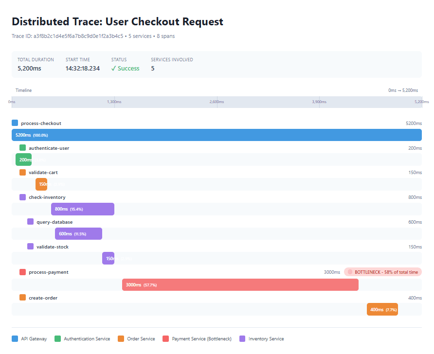
Traces answer critical questions that metrics and logs cannot address individually: Why is this particular request slow? Which service in the chain is causing the bottleneck? How do failures in one service cascade to others? What’s the dependency structure of our system for this particular operation?
The power of tracing becomes especially evident in complex scenarios. Consider an e-commerce checkout process that touches ten different services. When a customer reports that their checkout took twelve seconds—far longer than the typical two-second experience—metrics might show that your payment service had elevated latency during that period. However, the trace reveals that the delay actually originated in a third-party address verification API that timed out after ten seconds, causing multiple retries. This level of detail would be nearly impossible to discover through metrics or logs alone, as it requires understanding the causal chain and timing relationships between services.
Each span in a trace captures timing information, service and operation names, contextual attributes, and links to related spans. Spans form parent-child relationships that create a tree structure representing the complete request flow. Modern tracing implementations also support span events for significant occurrences within a span and span links for connecting related but non-hierarchical operations, such as batch processing or asynchronous workflows.
The three pillars work synergistically. Metrics provide the high-level view that triggers alerts when something goes wrong. Traces help you identify which specific requests are problematic and which services are involved. Logs provide the detailed context needed to understand exactly what went wrong and why. Together, they enable engineers to move from “We have a problem” to “Here’s exactly what’s wrong and how to fix it” in minutes rather than hours or days.
2. OpenTelemetry and Standardization
The observability landscape was once a fragmented ecosystem with competing proprietary formats, vendor-specific agents, and incompatible instrumentation libraries. Adopting a new observability platform often meant rewriting instrumentation code throughout your application, creating vendor lock-in and slowing innovation. OpenTelemetry emerged as the solution to this fragmentation—an open-source, vendor-neutral standard for collecting, processing, and exporting telemetry data.
What is OpenTelemetry?
OpenTelemetry, commonly abbreviated as OTel, represents a collaborative effort to create a unified standard for observability instrumentation. Born from the merger of two earlier projects—OpenTracing (focused on distributed tracing) and OpenCensus (focused on metrics and tracing)—in 2019, it has rapidly gained adoption across the industry. Major technology companies including Google, Microsoft, Amazon, and observability vendors like Datadog, New Relic, and Dynatrace all contribute to and support the project.
The framework provides several key components. First, it offers consistent APIs across multiple programming languages, ensuring that instrumentation patterns learned in Java apply equally well to Go, Python, or JavaScript. Second, it provides SDKs that implement these APIs with production-ready features like batching, retry logic, and resource detection. Third, it includes auto-instrumentation capabilities that automatically capture telemetry from popular frameworks and libraries without code changes. Fourth, it offers flexible exporters that can send data to virtually any observability backend. Finally, it establishes semantic conventions that ensure consistent naming and structure for common operations across different languages and frameworks.
The value proposition is compelling: write instrumentation once using OpenTelemetry, then export to any compatible backend. Want to evaluate whether Prometheus or Datadog offers better value for your use case? Switch backends by changing configuration, not code. Need to send the same telemetry data to multiple systems simultaneously? Configure multiple exporters. This flexibility fundamentally changes the economics and risk profile of observability investments.
The OpenTelemetry Architecture
OpenTelemetry’s architecture consists of several layers. At the application level, instrumentation code uses the OpenTelemetry API to create spans, record metrics, and emit logs. This instrumentation can be automatic (using the Java agent or framework integrations) or manual (explicit API calls in your code). The SDK collects this telemetry data and processes it according to configuration, handling concerns like sampling, batching, and resource attribution.
Telemetry data then flows to the OpenTelemetry Collector, an optional but recommended component that acts as a telemetry data pipeline. The Collector can receive data from multiple sources, process it through various processors (for filtering, transforming, enriching, or sampling), and export it to multiple destinations. This architecture decouples applications from backend systems, allowing centralized configuration of data routing and transformation.
For example, you might configure the Collector to send all error traces to your premium observability platform for detailed analysis while sending only sampled successful traces to a cost-effective long-term storage system. You could enrich all telemetry with environment-specific attributes, scrub sensitive data before export, or aggregate metrics to reduce cardinality.
Implementing OpenTelemetry in Java Applications
Java applications can adopt OpenTelemetry through several approaches, each offering different trade-offs between ease of implementation and control. The zero-code approach uses the OpenTelemetry Java agent, a JAR file that attaches to your application at startup and automatically instruments popular frameworks. This approach requires no application code changes and works with existing applications.
To use the Java agent, you download the latest release and start your application with additional JVM arguments. The agent automatically detects frameworks like Spring Boot, JDBC, HTTP clients, and messaging systems, capturing traces for incoming requests and outgoing calls. You configure the service name, exporter endpoints, and sampling strategies through system properties or environment variables.
For applications requiring more control, the SDK-based approach allows programmatic configuration. You add OpenTelemetry dependencies to your build configuration and create SDK instances with custom settings. This approach enables fine-grained control over sampling strategies, span processors, resource attributes, and exporter configurations. It’s particularly useful for applications with special requirements or those using less common frameworks.
Manual instrumentation provides the highest level of control, allowing you to create custom spans for business-critical operations, add domain-specific attributes, and implement specialized error handling. You obtain a Tracer instance from the OpenTelemetry SDK and use it to create spans around important operations. Each span can include custom attributes that provide business context, making traces more useful for understanding application behavior.
The Standardization Advantage
OpenTelemetry’s vendor neutrality provides significant strategic and operational benefits. The most obvious is avoiding vendor lock-in—your instrumentation investment remains valuable regardless of which observability platform you choose. This creates negotiating leverage and enables you to optimize costs by comparing offerings from multiple vendors.
Standardization also accelerates innovation. Because OpenTelemetry is community-driven with contributions from major tech companies, it evolves rapidly to support new technologies and patterns. Auto-instrumentation for new frameworks typically appears quickly, and best practices emerge through community collaboration rather than vendor advocacy.
The unified approach across telemetry types simplifies development and operations. Instead of learning separate systems for metrics, logs, and traces, teams work with a consistent API and mental model. This reduces training time and cognitive load while increasing the likelihood that instrumentation is implemented correctly.
Finally, OpenTelemetry enables interoperability between tools. You might use Prometheus for metrics, Jaeger for traces, and Elasticsearch for logs—all consuming data from the same OpenTelemetry instrumentation. As your needs evolve, you can add or replace tools without touching application code.
3. Distributed Tracing in Microservices
Microservices architectures deliver significant benefits in terms of development velocity, scalability, and organizational autonomy. However, they introduce observability challenges that traditional monitoring approaches cannot adequately address. When a single user request might touch a dozen services, each running across multiple instances in different data centers, understanding system behavior requires distributed tracing.
The Distributed Systems Challenge
Consider a typical e-commerce platform built with microservices. A single checkout operation might involve the following sequence: the API Gateway receives the HTTPS request and performs rate limiting, the Authentication Service validates the user’s session token and retrieves their profile, the Cart Service fetches items from Redis and calculates quantities, the Inventory Service checks stock availability across multiple warehouses by querying a distributed database, the Pricing Service applies user-specific discounts by calling a rules engine, the Payment Service processes the transaction through a third-party payment gateway, the Order Service creates order records in a transactional database, the Shipping Service schedules delivery by calling a logistics API, and finally the Notification Service sends confirmation emails through a messaging queue.
If this checkout takes eight seconds—four times longer than expected—which service is responsible? Without distributed tracing, engineers face an investigation nightmare. They might start by checking service-level metrics, discovering that several services show elevated latency. They then examine logs across multiple services, trying to correlate timestamps and request identifiers that may not be consistent. They might attempt to reproduce the issue in a staging environment, only to find it doesn’t occur there due to differences in data volume, network latency, or third-party behavior. Hours or days might pass before identifying the root cause.
Distributed tracing solves this problem by creating a unified view of the entire request journey. Every operation—from the initial API call through every service hop, database query, and external API call—becomes a span within a single trace. The trace reveals not just which services were involved, but exactly how long each operation took, which operations ran sequentially versus concurrently, and where the actual bottleneck occurred.
Core Concepts of Distributed Tracing
Distributed tracing relies on several fundamental concepts. The trace represents the complete journey of a request through the system, assigned a globally unique identifier that follows the request everywhere it goes. Each trace consists of multiple spans, representing individual units of work such as handling an HTTP request, executing a database query, or calling another service.
Spans form parent-child relationships that create a tree structure. When Service A calls Service B, Service A’s span becomes the parent of Service B’s span. This hierarchy reveals the dependency structure and execution flow of your system. Each span captures timing information including start time and duration, operation names that describe what work occurred, service names identifying which component performed the work, and custom attributes providing operation-specific context.
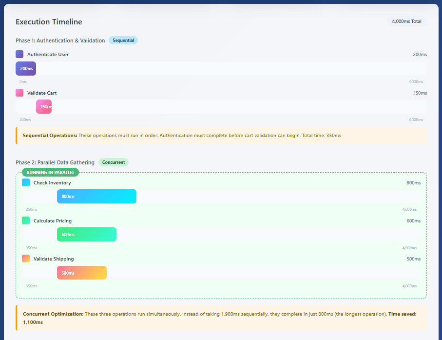
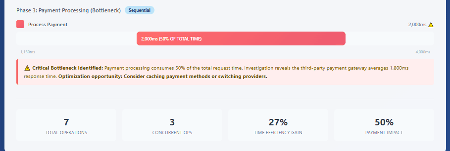
A detailed trace timeline showing concurrent vs sequential operations. Display a parent span “process-checkout” (total 4000ms) with multiple child spans. Show some operations running sequentially (authenticate-user 200ms → validate-cart 150ms) and others running concurrently (check-inventory 800ms parallel with calculate-pricing 600ms parallel with validate-shipping 500ms). Then show process-payment 2000ms as the obvious bottleneck. Use color coding to distinguish different services and include small annotations showing the percentage of total time each operation consumed.

Context propagation enables distributed tracing by passing trace and span identifiers across service boundaries. Modern implementations use the W3C Trace Context standard, which defines HTTP headers that carry trace information. When Service A calls Service B, it includes these headers in the HTTP request. Service B extracts them, creates a new child span linked to Service A’s span, and continues propagating the context to any services it calls.
Sampling Strategies for Production Systems
Recording every single trace in a high-traffic production system is prohibitively expensive both in terms of performance overhead and storage costs. A system handling ten thousand requests per second generates ten thousand traces per second, or 864 million traces per day. Sampling strategies reduce this volume while maintaining observability effectiveness.
Head-based sampling makes the recording decision at the start of the trace, typically using a random probability. For example, a 1% sample rate means that out of every hundred requests, one is traced in full detail while the other ninety-nine are not instrumented. This approach is simple, predictable, and has minimal performance impact. However, it suffers from a significant drawback: you might miss interesting traces. If only one request out of a thousand fails, and you’re sampling at 1%, you’ll likely miss that failure in your trace data.
Tail-based sampling addresses this limitation by deferring the recording decision until after the trace completes. The system temporarily buffers all spans for a trace, then decides whether to keep or discard the entire trace based on its characteristics. For example, you might keep all traces with errors, all traces slower than five seconds, and a random 0.1% sample of everything else. This ensures you capture interesting behavior while still dramatically reducing overall volume.
The challenge with tail-based sampling is complexity. Spans for a single trace might arrive at the collection system from dozens of services over several seconds. You need a stateful component—typically the OpenTelemetry Collector—that can buffer spans, group them by trace ID, wait for trace completion, and then make sampling decisions. This adds infrastructure complexity and resource requirements compared to head-based sampling.
Adaptive sampling represents an advanced approach that adjusts sampling rates dynamically based on observed patterns. For example, you might normally sample successful requests at 1% but automatically increase to 10% when error rates rise. You could sample differently based on customer tier, geographic region, or feature flags. Some systems use algorithms that ensure representative sampling across all endpoints while adapting to traffic patterns.
Production systems often combine multiple strategies. A common pattern is to use head-based sampling at a low rate for routine traffic while implementing tail-based rules to capture all errors, slow requests, and requests from specific test accounts or premium users. This balances cost control with comprehensive coverage of interesting scenarios.
Implementing Effective Tracing
Effective distributed tracing requires more than just enabling auto-instrumentation. Several practices separate helpful traces from overwhelming noise. First, use meaningful span names that clearly describe the operation. Generic names like “process” or “handle” provide little value, while specific names like “charge-credit-card” or “validate-inventory-availability” immediately communicate what the span represents.
Second, add rich contextual attributes to spans. While timing information tells you that an operation took two seconds, attributes tell you why. For a payment processing span, include the payment method, amount, currency, customer tier, and transaction type. For a database query span, include the table name, query type, and number of rows affected. These attributes enable powerful filtering and analysis, such as identifying that payment failures correlate with a specific card issuer or that slow queries all involve a particular table.
Third, properly handle errors and exceptions. When an exception occurs, record it on the relevant span along with contextual information about what was being attempted. Mark the span as having encountered an error using the appropriate status code. This enables error tracking and makes it easy to find traces containing failures.
Fourth, be thoughtful about span granularity. Creating too few spans provides insufficient visibility into where time is spent within a service. Creating too many spans generates overhead and creates visual clutter in trace viewers. A reasonable rule of thumb is to create spans for operations that typically take more than a few milliseconds, such as external service calls, database queries, significant business logic operations, and message queue interactions.
Analyzing Traces for Performance Optimization
Distributed traces become truly valuable when used systematically to identify and resolve performance issues. The waterfall view provided by most tracing systems reveals several common patterns. Sequential bottlenecks occur when operations that could run in parallel execute sequentially instead, often due to synchronous code patterns. The trace shows operations stacked vertically with no overlap, revealing optimization opportunities through parallelization or asynchronous processing.
Latency spikes in individual services become immediately visible when comparing traces of fast and slow requests. If a normally 50-millisecond operation occasionally takes 500 milliseconds, the trace attributes often reveal the cause—perhaps queries involving specific customers hit un-indexed database columns, or requests during certain time windows encounter rate limiting from downstream services.
Cascading failures show how problems in one service propagate through the system. A trace might reveal that when the Inventory Service experiences high latency, it causes the Order Service to time out, which causes the API Gateway to retry, which increases load on the Inventory Service, creating a positive feedback loop. Understanding these cascades is essential for building resilient systems.
Traces also reveal unexpected dependencies. You might discover that your checkout process intermittently calls a recommendation engine that wasn’t supposed to be in the critical path, or that certain requests trigger synchronous calls to a batch processing system that should only be accessed asynchronously. These discoveries lead to architectural improvements.
4. Metrics That Matter for Java Applications
Effective observability requires focusing on metrics that provide actionable insights while avoiding metric overload. The challenge isn’t collecting metrics—modern frameworks make that trivial—but rather identifying which metrics actually indicate problems and warrant engineering attention.
The RED Method for Request-Driven Services
The RED method, popularized by Tom Wilkie of Grafana Labs, provides a simple but powerful framework for monitoring request-driven services. RED stands for Rate, Errors, and Duration—three metrics that together provide a comprehensive health snapshot for any service that processes requests.
Rate measures requests per second, providing visibility into traffic patterns and capacity utilization. Sudden drops in rate might indicate upstream problems or outages. Sudden increases might trigger capacity scaling or indicate abuse. Comparing current rate to historical patterns helps distinguish normal variation from anomalies. Rate metrics should be broken down by important dimensions such as endpoint, HTTP method, and customer tier to enable granular analysis.
Errors measure failed requests per second, typically as a count and as a percentage of total requests. Not all errors are equal—a 400 Bad Request error indicates client problems, while a 500 Internal Server Error indicates service issues. Tracking error rates by status code category, error type, and affected operation enables rapid problem identification. A sudden spike in 502 Bad Gateway errors suggests downstream service problems, while increasing 503 Service Unavailable errors indicate capacity exhaustion.
Duration measures request latency, best represented as a distribution rather than a simple average. The average response time might be 100 milliseconds, but if 5% of requests take five seconds, users will perceive the service as slow. Percentile metrics provide this visibility—p50 (median) shows typical performance, p95 shows what slower requests experience, and p99 reveals tail latency that affects a small but significant portion of users. Duration metrics should track multiple percentiles and be broken down by endpoint to identify which operations are slow.
These three metrics answer fundamental questions during incidents. If alerts fire, you first check which metrics changed. Rising error rates indicate failures to investigate. Increasing duration suggests performance degradation. Dropping rates might indicate upstream problems or suggest that errors are happening so fast that downstream services aren’t seeing traffic. The RED method provides a mental model for incident investigation that works across all request-driven services.
The USE Method for Resource Monitoring
While RED focuses on request-driven services, the USE method developed by Brendan Gregg applies to physical resources like CPU, memory, disk, and network interfaces. USE stands for Utilization, Saturation, and Errors—three metrics that together reveal resource health.
Utilization measures the percentage of time a resource is busy performing useful work. High CPU utilization might indicate compute-intensive workloads or inefficient code. High memory utilization could suggest memory leaks or simply that your application’s working set is growing. Utilization metrics help determine whether you need more capacity or whether optimization would be more effective.
Saturation measures the degree of queued work that cannot be serviced. When a resource reaches maximum utilization, additional work must wait. CPU saturation manifests as increasing load averages beyond core count. Memory saturation shows up as swapping or increasing page faults. Thread pool saturation appears as growing queue lengths. Saturation metrics often prove more useful than utilization for identifying performance problems, as they directly indicate resource exhaustion.
Errors count resource-related failures such as network packet drops, disk read errors, or out-of-memory conditions. These metrics are critical for distinguishing performance problems from reliability problems. If your application is slow due to high utilization and saturation but has no errors, you need more capacity. If you’re seeing errors, you have reliability issues requiring different solutions.
Critical JVM Metrics
Java applications require monitoring of JVM-specific metrics that don’t apply to other runtime environments. Understanding these metrics is essential for maintaining application health and performance.
Garbage collection metrics provide crucial insights into memory management. GC pause duration measures how long the application stopped executing application code while the collector ran. Long or frequent pauses directly impact user experience. Memory allocation rate shows how quickly the application creates new objects. A high allocation rate leads to frequent GC cycles and can indicate inefficient object creation patterns. Promotion rate tracks how much data moves from young generation to old generation. Rapidly increasing promotion suggests memory leaks or that objects aren’t being released as expected.
Heap usage metrics show current memory consumption relative to maximum heap size. Consistently high heap usage approaching maximum indicates potential memory pressure. Monitoring both used heap and committed heap reveals whether the JVM is already using allocated memory or requesting more from the operating system.
Thread metrics reveal concurrency behavior. Live thread count shows how many threads currently exist. Rapidly increasing thread counts might indicate thread leaks. Blocked thread count reveals contention issues—threads waiting to acquire locks or resources. High blocked thread counts often correlate with performance problems and warrant investigation. Thread state distribution shows what threads are doing—sleeping, waiting, running, or blocked.
Class loading metrics track how many classes are loaded and whether class loading frequency changes over time. Unexpected increases in class loading might indicate inefficient code reloading or classloader leaks.
Connection pool metrics matter for applications using databases or external services. Pool size, active connections, and queue length reveal whether connection pools are properly sized. Consistently maxed-out pools cause request queueing and increased latency. Monitoring connection acquisition time helps identify when pool exhaustion is impacting performance.
Application-Specific Business Metrics
Beyond infrastructure and JVM metrics, instrument operations that matter to your business. For an e-commerce system, track orders placed per minute, average order value, payment success rate, and shopping cart abandonment rate. For a SaaS application, monitor active users, feature usage, API calls per customer, and subscription changes.
Business metrics serve multiple purposes. They provide early warning of problems that don’t trigger technical alerts—for example, payment success rate dropping from 98% to 95% might not trigger error rate alerts but represents significant revenue loss. They enable product teams to understand feature adoption and usage patterns. They facilitate communication with non-technical stakeholders by providing metrics that directly relate to business outcomes.
The key is instrumenting operations at the business logic layer, not just at the HTTP request layer. When a user completes checkout, emit a metric with attributes for order value, payment method, customer segment, and whether discounts were applied. When a background job processes data, emit metrics for items processed, processing duration, and failure counts. This granular instrumentation enables sophisticated analysis connecting technical performance to business outcomes.
Managing Metric Cardinality
Metric cardinality—the number of unique label combinations—dramatically impacts storage costs and query performance. A metric with three labels, each having ten possible values, has one thousand potential unique time series (10 × 10 × 10). A metric with five labels having one hundred possible values each has ten billion potential combinations.
High cardinality arises from using unbounded values as labels. User IDs, transaction IDs, IP addresses, and timestamps create unique label combinations for every event. A payment processed metric with a user_id label might have millions of unique time series, overwhelming your monitoring system and making the metric unusable.
The solution is using bounded categorical values for labels while storing unbounded values in traces and logs. Instead of labeling a payment metric with user_id, use user_tier (free, premium, enterprise). Instead of ip_address, use geographic_region. Instead of timestamp, use time_of_day_category (night, morning, afternoon, evening). This approach maintains useful dimensionality while keeping cardinality manageable.
As a rule of thumb, keep label cardinality to hundreds or low thousands of unique combinations per metric. Monitor your metric cardinality and identify metrics consuming disproportionate storage or causing query performance issues. Many monitoring platforms provide cardinality analysis tools to help identify problematic metrics.
5. Log Aggregation Strategies
In distributed systems, logs scattered across dozens or hundreds of service instances become useful only when aggregated into a centralized, searchable system. Effective log aggregation transforms fragmented diagnostic data into actionable insights, but it requires careful strategy to balance comprehensiveness with cost and performance.
From Plain Text to Structured Logging
Traditional Java logging wrote human-readable text messages to files. While this works for simple applications, it creates significant challenges at scale. Plain text logs require complex regular expressions to parse, making automated analysis difficult. Different developers format logs inconsistently, creating parsing nightmares. Extracting structured data like user IDs or transaction amounts requires fragile string manipulation.
Modern logging practices favor structured formats, typically JSON, that maintain human readability while enabling powerful machine processing. Structured logs include consistent fields that log aggregation systems can automatically index and query. Instead of parsing text to extract a user ID, you query a structured field directly.
The transformation is straightforward with modern Java logging frameworks. Libraries like Logstash Logback Encoder generate JSON-formatted logs with minimal configuration changes. Each log statement can include structured key-value pairs that become searchable fields in your log aggregation system.
The benefits compound in distributed systems. When every service logs in a consistent structured format, you can query across all services simultaneously. Questions like “Show me all ERROR logs from any service where the user was user-12345 and the transaction amount exceeded one thousand dollars” become simple queries rather than complex scripting exercises.
Integrating Logs with Traces
The most powerful debugging workflows emerge when logs integrate seamlessly with distributed traces. During an incident, engineers typically start with metrics to identify the problem scope, then examine traces to understand request flow and identify problematic services, and finally need logs to see detailed error messages and diagnostic information.
The connection point is trace and span identifiers. When every log entry includes the trace ID and span ID from the current context, log aggregation systems can link logs to traces bidirectionally. Viewing a slow trace, you can jump directly to logs from any span in that trace. Examining an error log, you can navigate to the full trace context showing what led to that error.
Implementation requires adding trace context to logging’s Mapped Diagnostic Context (MDC), which automatically includes configured values in every log statement. When a request enters your service, extract the trace ID and span ID from the current OpenTelemetry span and add them to MDC. Clear them when the request completes. This small change enables powerful cross-cutting queries and navigation.
The integrated approach dramatically reduces mean time to resolution during incidents. Instead of separately investigating traces and logs, engineers work with a unified view of what happened. They can see that a particular trace was slow, identify which span was problematic, and immediately view the detailed error logs from that operation without manual correlation.
Log Level Management
Log volume directly impacts storage costs, query performance, and incident investigation effectiveness. Appropriate log level usage is essential for managing costs while maintaining diagnostic value. The standard log levels serve distinct purposes with different production characteristics.
ERROR level logs capture failures requiring immediate attention, such as uncaught exceptions, failed database transactions, or critical business operations that failed. Production systems should generate relatively few ERROR logs—if errors are common enough to be noise, they’re not actually errors but expected conditions that should be logged at WARN or INFO level. ERROR logs should always include sufficient context to diagnose the problem without requiring additional information.
WARN level logs indicate concerning conditions that don’t prevent continued operation but warrant attention. Examples include using deprecated APIs, retrying failed operations, receiving unexpected but handleable input, or approaching resource limits. WARN logs should occur more frequently than ERROR but still represent unusual conditions.
INFO level logs capture significant business events and operational milestones—application startup and shutdown, configuration changes, user authentication, order processing, payment completion, and job completion. INFO logs provide the operational narrative of what your application is doing. They should be meaningful but not overwhelming. A service handling one thousand requests per second shouldn’t log every request at INFO level but might log aggregated summaries.
DEBUG and TRACE levels provide detailed diagnostic information used during development and troubleshooting but typically disabled in production due to volume. DEBUG might log method parameters, query results, and intermediate calculations. TRACE captures very detailed information like method entry and exit. Production systems enable these levels temporarily for specific troubleshooting sessions, then disable them to control volume.
Sampling and Filtering Strategies
Even with appropriate log levels, high-traffic applications generate overwhelming log volumes. A service handling one million requests per day, logging even two INFO-level lines per request, generates two million log lines daily—about 600 million per month. At typical log storage costs, this becomes expensive quickly.
Sampling strategies reduce volume while retaining diagnostic value. The simplest approach is probabilistic sampling, logging only a percentage of events. For routine successful operations, logging 1% of events typically provides sufficient visibility into patterns and trends while reducing volume by 99%. The key is ensuring you don’t sample errors or unusual conditions—always log problems in full detail.
Conditional sampling applies different rates to different scenarios. Log all premium customer requests at full detail while sampling free-tier customers at 1%. Log all requests exceeding a duration threshold in full detail while sampling fast requests. Log all requests involving financial transactions completely while sampling read-only operations. This approach ensures you have detailed logs for important scenarios while controlling overall volume.
Aggregation at the source reduces repetitive logs. Instead of logging every successful cache hit, periodically log aggregated statistics: “In the last 60 seconds, cache had 10,000 hits (98% hit rate), 200 misses, 50 evictions.” This one log line replaces ten thousand individual logs while still providing visibility into cache behavior.
Log filtering drops logs matching specific patterns entirely. Successfully processed health check requests from load balancers might generate millions of logs with no diagnostic value. Filter them at the source rather than paying to ingest, store, and index them. Similarly, DEBUG-level logs from chatty libraries can be filtered unless specifically needed for troubleshooting.
Retention Policies and Tiered Storage
Different log types require different retention periods based on their diagnostic and compliance value. Recent logs need to be immediately queryable for active investigations. Older logs might be acceptable with slower query performance. Very old logs might only need to exist for compliance purposes without any query capability.
Implement tiered retention policies that balance accessibility with cost. Keep the most recent 7-14 days in hot storage with sub-second query performance. Move 15-90 day old logs to warm storage with acceptable query performance at lower cost. Archive logs older than 90 days to cold storage for compliance purposes only, with very slow query performance or no query capability at all.
Different log categories warrant different retention. Application logs capturing routine operations might need only 30 days of retention. Audit logs tracking security-relevant actions might require seven years for regulatory compliance. Error logs might keep 180 days for pattern analysis. Access logs tracking HTTP requests might retain 90 days for security investigations.
Most log aggregation platforms support automated lifecycle policies that transition logs between storage tiers based on age. Configure these policies to match your requirements, balancing diagnostic needs against storage costs. Remember that searching cold storage is often prohibitively slow or expensive, so ensure you’ve transitioned logs before they’re needed for investigations.
6. Cost-Effective Observability Approaches
Observability platforms can consume significant budgets, especially at scale. Understanding cost drivers and optimization strategies enables comprehensive visibility without excessive spending.
Understanding Observability Costs
Observability costs stem from several sources. Data ingestion charges based on volume—every log line, metric data point, and trace span you send to your platform incurs cost. Storage charges accumulate based on how long you retain data and in which storage tier. Query execution costs arise from complex searches and aggregations, especially over large time ranges. Platform licensing might be based on host count, data volume, user seats, or feature access. Alert and dashboard creation might incur additional charges.
For a typical application, logs often dominate costs. A single moderately busy service might generate gigabytes of log data daily. Distributed tracing is typically second due to the rich contextual data in spans. Metrics, being aggregated numerical data, usually consume the least storage despite their high value for monitoring.
Understanding these cost drivers informs optimization strategies. Reducing log volume by 50% through better sampling might cut observability costs by 30% overall. Optimizing trace sampling affects both ingestion and storage costs. Managing metric cardinality prevents exponential cost growth as you add dimensions.
Strategic Sampling
Intelligent sampling dramatically reduces costs while maintaining observability effectiveness. The goal is retaining visibility into interesting behavior while reducing the volume of routine operations.
For traces, implement multi-tier sampling. Use very low rates for routine successful requests—perhaps 0.1% to 1%. Apply higher rates to important customer segments, perhaps 10% for premium customers. Always capture error traces and slow traces using tail-based sampling. This approach might reduce overall trace volume by 95% while ensuring you still capture every anomalous request.
For logs, apply similar strategies. Sample routine INFO-level logs from successful operations at 1% to 5%. Always capture WARN and ERROR logs completely. Apply higher sampling rates to critical paths like payment processing or authentication. Log aggregated summaries rather than individual events for high-frequency operations.
For metrics, focus on cardinality management rather than sampling, as metrics are already aggregated. Limit label dimensions to bounded categorical values. Consider aggregating some metrics at collection time—instead of tracking per-endpoint latency for hundreds of endpoints, perhaps track only the top ten busiest endpoints explicitly and group others into an “other” category.
Hybrid Approaches
Many organizations adopt hybrid observability strategies, using different tools for different purposes based on their cost-value profiles. Open-source tools like Prometheus for metrics and Jaeger for traces handle high-volume data cost-effectively. Commercial platforms provide advanced features for the subset of data requiring sophisticated analysis.
For example, you might send all metrics to self-hosted Prometheus, all traces to self-hosted Jaeger, and only ERROR-level logs plus sampled INFO logs to a commercial log aggregation platform. This reduces commercial platform costs by 90% while maintaining comprehensive metrics and traces in cost-effective systems.
Another approach uses commercial platforms for production environments requiring 24/7 support and SLAs, while using open-source tools for development and staging environments. This optimizes spending where reliability matters most while controlling costs in lower environments.
Geographic optimization routes data efficiently. Services deployed globally might send telemetry to regional collection points that aggregate and forward only relevant data to central platforms, reducing cross-region data transfer costs.
Retention Optimization
Storage costs accumulate quickly for long retention periods. Optimize retention based on diagnostic value over time. Recent data needs fast queries for active investigations. Older data might tolerate slower access. Very old data might only need to exist for compliance, never requiring queries.
Implement automated retention policies that delete or archive data based on age and type. Keep high-resolution metrics for seven days, then downsample to one-minute averages for 30 days, then five-minute averages for one year. Retain error logs longer than successful operation logs. Delete health check logs aggressively.
Consider selective retention based on importance. Always retain traces containing errors for 90 days. Sample or delete successful traces after 30 days. Retain logs from critical services longer than logs from less critical services.
7. Tools Comparison: Building Your Observability Stack
The observability tooling landscape offers numerous options across commercial and open-source solutions. Understanding the strengths, limitations, and cost profiles of major tools helps build an effective stack for your requirements.
Metrics: Prometheus and Grafana
Prometheus has become the de facto standard for metrics collection and storage in cloud-native environments. It uses a pull-based model, scraping metrics from instrumented applications at regular intervals. Prometheus excels at reliability, with minimal dependencies and simple deployment. Its time-series database handles high cardinality reasonably well, though it has limits. The query language, PromQL, provides powerful aggregation and analysis capabilities.
Grafana complements Prometheus perfectly, providing visualization and dashboarding. Grafana supports multiple data sources beyond Prometheus, enabling unified dashboards combining metrics, logs, and traces. Its templating system enables creating reusable dashboards that work across multiple services or environments. Alert routing integrations with PagerDuty, Slack, and other platforms complete the monitoring workflow.
The Prometheus-Grafana combination offers exceptional cost-effectiveness for metrics. Both are open source with no licensing costs. Infrastructure costs are predictable based on data volume and retention. Organizations running Kubernetes clusters can deploy Prometheus and Grafana with minimal additional infrastructure. Commercial offerings like Grafana Cloud provide hosted versions for teams preferring managed services.
Limitations include Prometheus’s single-node architecture, which constrains scalability, though recent federation and remote storage features address this. Long-term storage requires additional solutions, as Prometheus optimizes for recent data. High cardinality can still cause performance issues despite improvements.
Tracing: Jaeger and Zipkin
Jaeger, originally developed by Uber and now a CNCF project, provides distributed tracing collection, storage, and visualization. It supports OpenTelemetry natively, making it an excellent choice for standards-based tracing. Jaeger offers multiple storage backends including Cassandra, Elasticsearch, and Kafka, enabling scaling to large trace volumes. The UI provides intuitive trace visualization, making it easy to understand request flows and identify bottlenecks.
Zipkin, one of the earliest distributed tracing systems, remains popular for its simplicity and maturity. It provides similar capabilities to Jaeger with a different architectural approach. Both tools handle the core tracing use cases effectively, with Jaeger having momentum in the cloud-native community due to CNCF backing and active development.
For cost-conscious organizations, self-hosted Jaeger provides enterprise-grade tracing without licensing costs. Infrastructure costs scale with trace volume, but intelligent sampling keeps storage requirements manageable. Teams preferring managed services can use commercial offerings or hosted Jaeger services from various providers.
Limitations include the operational complexity of running and scaling backend storage. Elasticsearch-based storage requires careful tuning and can become expensive at large scale. Cassandra offers better scalability but more operational complexity. Query capabilities are focused on individual traces rather than complex aggregations across many traces.
Logging: ELK Stack
The ELK Stack—Elasticsearch, Logstash, and Kibana—has long been a popular choice for log aggregation and analysis. Elasticsearch provides scalable, searchable storage for structured logs. Logstash collects and transforms log data from various sources. Kibana offers visualization and query interfaces. More recently, Elastic has positioned their Observability solution as a complete platform including metrics and traces alongside logs.
Elasticsearch excels at full-text search and complex queries across massive log volumes. Its distributed architecture scales horizontally to petabyte-scale deployments. Kibana’s query language and visualization capabilities enable sophisticated log analysis. Integration with various log shippers beyond Logstash, including Filebeat and Fluentd, provides deployment flexibility.
Cost considerations are significant for the ELK Stack. Self-hosting requires substantial infrastructure for Elasticsearch clusters, especially at scale. Elasticsearch resource requirements grow with data volume and query complexity. Commercial Elastic Cloud offerings simplify operations but charge based on deployment size. Index management, retention policies, and query optimization require expertise.
Alternatives like Grafana Loki offer simpler, more cost-effective logging focused on integrating with existing metrics and tracing tools. Loki deliberately trades query flexibility for cost efficiency, indexing only labels rather than full log content. For many use cases, this tradeoff is acceptable and dramatically reduces storage costs.
Comprehensive Commercial Platforms
Commercial observability platforms like Datadog, New Relic, and Dynatrace provide integrated solutions combining metrics, traces, and logs with advanced features like automatic anomaly detection, AI-powered insights, and sophisticated alerting. These platforms reduce operational overhead, provide excellent user experiences, and offer features difficult to replicate with open-source tools.
The value proposition includes rapid deployment without operating infrastructure, automatic instrumentation reducing development effort, unified interfaces across telemetry types, advanced analytics and machine learning features, and comprehensive vendor support. For many organizations, especially those without dedicated platform teams, these benefits justify the premium pricing.
Cost is the primary consideration. Commercial platforms typically charge based on data volume, host count, or custom metrics, with pricing escalating significantly at scale. Organizations handling terabytes of telemetry data might face six or seven-figure annual bills. Understanding pricing models and implementing data management strategies becomes critical.
Hybrid approaches can optimize costs. Use commercial platforms for critical production services while using open-source tools for development environments. Send full trace volumes to self-hosted systems while sending only error traces to commercial platforms for advanced analysis. Route different telemetry types to different platforms based on analysis needs.
Making Tool Selections
Selecting observability tools requires balancing multiple factors. Consider your team’s expertise—operating Elasticsearch clusters requires different skills than managing Prometheus. Evaluate current and projected data volumes, as cost profiles vary significantly at different scales. Assess required features beyond basic collection and visualization, such as anomaly detection or synthetic monitoring.
Integration with existing infrastructure matters. If already running Kubernetes, Prometheus and Jaeger integrate naturally. If heavily using AWS, CloudWatch and X-Ray might reduce operational complexity. If committed to open standards, prioritize OpenTelemetry-compatible tools.
Start with specific use cases rather than comprehensive coverage. Implement metrics first to establish monitoring and alerting. Add distributed tracing for performance optimization. Integrate logging last, as it typically has the highest cost and operational complexity. Prove value incrementally rather than deploying complete observability stacks upfront.
Maintain flexibility through standardization. By using OpenTelemetry for instrumentation, you avoid vendor lock-in and can evaluate alternatives as your needs evolve. The observability landscape changes rapidly, and what’s optimal today might not be tomorrow.
8. Conclusion: Key Takeaways
Throughout this comprehensive exploration of observability in Java applications, we’ve examined how the three pillars—metrics, logs, and traces—work together to provide complete visibility into distributed systems. We’ve seen how OpenTelemetry standardization enables vendor-neutral instrumentation that provides flexibility and avoids lock-in. We’ve explored how distributed tracing reveals request flows and bottlenecks in microservices architectures that would be nearly impossible to diagnose through other means. We’ve identified the specific metrics that matter most for Java applications, from the RED method for services to USE method for resources, while understanding how to manage cardinality to control costs. We’ve discussed log aggregation strategies that balance comprehensiveness with practical cost considerations through sampling, structured logging, and integration with traces. Finally, we’ve compared popular tools and explored cost-effective approaches that deliver enterprise-grade observability without excessive spending.
The key lesson is that effective observability is not about collecting every possible data point, but rather about strategically instrumenting systems to capture the information needed to understand, diagnose, and optimize production behavior. By combining the right tools, thoughtful sampling strategies, and integration between metrics, logs, and traces, teams can build observability systems that provide rapid incident response, enable proactive optimization, and support confident deployment of complex distributed Java applications.