When working with data, one of the most common tasks involves performing calculations across groups or windows of records. Whether you’re calculating running totals, ranking values, or computing moving averages, both SQL and Python offer powerful tools for these operations. SQL’s OVER clause and pandas‘ groupby and rolling methods represent two different philosophical approaches to the same fundamental problem, each with its own strengths and trade-offs.
Getting Started with Sample Data
To follow along with all the examples in this article, you’ll need sample datasets. I’ve provided two tables: a sales table for time-series operations and an employees table for ranking examples. You can set this up in two ways depending on your preference.
Option A: Using SQLite (Recommended for Beginners)
SQLite requires no server setup and works perfectly for learning. Here’s a complete Python script that creates the database, loads sample data, and runs all examples:
import sqlite3
import pandas as pd
from datetime import datetime, timedelta
import random

# Create SQLite database
conn = sqlite3.connect('sample_data.db')
cursor = conn.cursor()

# Create sales table
cursor.execute('''
CREATE TABLE IF NOT EXISTS sales (
    product_category TEXT,
    sale_date DATE,
    sale_amount DECIMAL(10,2),
    product_id INTEGER
)
''')

# Create employees table
cursor.execute('''
CREATE TABLE IF NOT EXISTS employees (
    employee_name TEXT,
    department TEXT,
    salary DECIMAL(10,2)
)
''')

# Generate sample sales data
categories = ['Electronics', 'Clothing', 'Home & Garden', 'Sports']
start_date = datetime(2024, 1, 1)
sales_data = []

for i in range(500):
    category = random.choice(categories)
    date = start_date + timedelta(days=random.randint(0, 365))
    amount = round(random.uniform(50, 500), 2)
    product_id = random.randint(1, 20)
    sales_data.append((category, date.strftime('%Y-%m-%d'), amount, product_id))

cursor.executemany('INSERT INTO sales VALUES (?, ?, ?, ?)', sales_data)

# Generate sample employee data
employees_data = [
    ('Alice Johnson', 'Engineering', 95000),
    ('Bob Smith', 'Engineering', 87000),
    ('Carol White', 'Engineering', 92000),
    ('David Brown', 'Sales', 75000),
    ('Eve Davis', 'Sales', 82000),
    ('Frank Miller', 'Sales', 75000),
    ('Grace Wilson', 'Marketing', 68000),
    ('Henry Moore', 'Marketing', 71000),
    ('Iris Taylor', 'Marketing', 73000),
    ('Jack Anderson', 'Engineering', 105000),
    ('Kate Thomas', 'Sales', 89000),
    ('Leo Martinez', 'Engineering', 87000)
]

cursor.executemany('INSERT INTO employees VALUES (?, ?, ?)', employees_data)

conn.commit()
print("Database created successfully! File: sample_data.db")
print(f"Sales records: {len(sales_data)}")
print(f"Employee records: {len(employees_data)}")

# Verify data
print("\nSample sales data:")
print(pd.read_sql("SELECT * FROM sales LIMIT 5", conn))
print("\nSample employee data:")
print(pd.read_sql("SELECT * FROM employees LIMIT 5", conn))

conn.close()
Save this as create_sample_data.py and run it. This creates a file called sample_data.db in your current directory.
Option B: CSV Files with Pandas
If you prefer working directly with pandas, here’s code to create CSV files:
import pandas as pd
from datetime import datetime, timedelta
import random

# Generate sales data
categories = ['Electronics', 'Clothing', 'Home & Garden', 'Sports']
start_date = datetime(2024, 1, 1)
sales_data = []

for i in range(500):
    category = random.choice(categories)
    date = start_date + timedelta(days=random.randint(0, 365))
    amount = round(random.uniform(50, 500), 2)
    product_id = random.randint(1, 20)
    sales_data.append({
        'product_category': category,
        'sale_date': date.strftime('%Y-%m-%d'),
        'sale_amount': amount,
        'product_id': product_id
    })

sales_df = pd.DataFrame(sales_data)
sales_df.to_csv('sales.csv', index=False)

# Generate employee data
employees_df = pd.DataFrame([
    {'employee_name': 'Alice Johnson', 'department': 'Engineering', 'salary': 95000},
    {'employee_name': 'Bob Smith', 'department': 'Engineering', 'salary': 87000},
    {'employee_name': 'Carol White', 'department': 'Engineering', 'salary': 92000},
    {'employee_name': 'David Brown', 'department': 'Sales', 'salary': 75000},
    {'employee_name': 'Eve Davis', 'department': 'Sales', 'salary': 82000},
    {'employee_name': 'Frank Miller', 'department': 'Sales', 'salary': 75000},
    {'employee_name': 'Grace Wilson', 'department': 'Marketing', 'salary': 68000},
    {'employee_name': 'Henry Moore', 'department': 'Marketing', 'salary': 71000},
    {'employee_name': 'Iris Taylor', 'department': 'Marketing', 'salary': 73000},
    {'employee_name': 'Jack Anderson', 'department': 'Engineering', 'salary': 105000},
    {'employee_name': 'Kate Thomas', 'department': 'Sales', 'salary': 89000},
    {'employee_name': 'Leo Martinez', 'department': 'Engineering', 'salary': 87000}
])
employees_df.to_csv('employees.csv', index=False)

print("CSV files created: sales.csv and employees.csv")
print(f"\nSales records: {len(sales_df)}")
print(f"Employee records: {len(employees_df)}")
Connecting to Your Data in Examples
For SQLite examples throughout this article:
import sqlite3
import pandas as pd

conn = sqlite3.connect('sample_data.db')
For CSV examples:
import pandas as pd

sales_df = pd.read_csv('sales.csv')
employees_df = pd.read_csv('employees.csv')
# Convert date column to datetime
sales_df['sale_date'] = pd.to_datetime(sales_df['sale_date'])
Now you’re ready to run all the examples in this article!
Understanding the Fundamentals
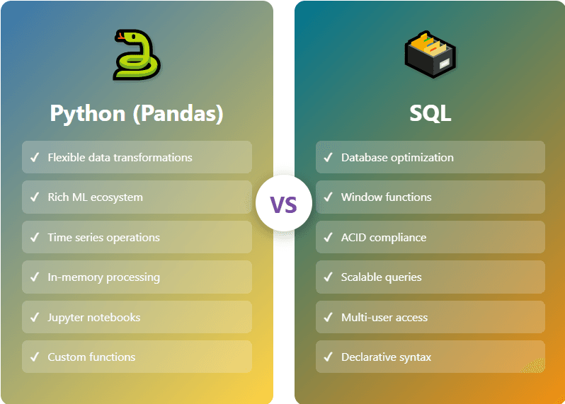
SQL window functions, introduced in the SQL:2003 standard, allow you to perform calculations across a set of rows that are related to the current row. Unlike traditional GROUP BY operations that collapse rows, window functions maintain the original row structure while adding computed columns. The OVER clause defines the window of rows for each calculation, making it possible to compute aggregates, rankings, and analytical functions without losing the granularity of your data.
Python’s pandas library takes a different approach through its groupby functionality, which splits data into groups, applies functions to each group, and combines the results. The rolling method provides time series specific operations that slide a window across your data. While conceptually similar to SQL window functions, pandas offers more flexibility in how you define and manipulate these operations, particularly when dealing with complex transformations.
Performance Characteristics
The performance debate between SQL window functions and pandas operations isn’t straightforward, as it depends heavily on your specific use case, data volume, and infrastructure. SQL databases are optimized for set-based operations and can leverage indexes, query optimization, and parallel processing capabilities built into the database engine. When you’re working with data that already lives in a database, keeping operations in SQL often means avoiding the overhead of data transfer and staying within an optimized execution environment.
Modern databases like PostgreSQL, SQL Server, and Oracle have highly optimized window function implementations that can handle millions of rows efficiently. The database engine can often push these operations down to the storage layer and take advantage of column-oriented storage or partitioning schemes. For operations on large datasets that don’t fit comfortably in memory, SQL’s ability to work with data on disk while maintaining reasonable performance is a significant advantage.
Pandas, on the other hand, operates entirely in memory and benefits from NumPy’s optimized C implementations for array operations. For datasets that fit in RAM, pandas can be extraordinarily fast, particularly for complex transformations that would require multiple passes in SQL. The ability to chain operations, use vectorized functions, and leverage Python’s rich ecosystem of scientific computing libraries can lead to more efficient workflows, even if individual operations might be slower than their SQL equivalents.
Syntax and Expressiveness
Let’s examine how these approaches differ in practice. Consider a sales dataset where we want to calculate the running total of sales for each product category. In SQL, this becomes quite elegant with the OVER clause:
SELECT
    product_category,
    sale_date,
    sale_amount,
    SUM(sale_amount) OVER (
        PARTITION BY product_category
        ORDER BY sale_date
        ROWS BETWEEN UNBOUNDED PRECEDING AND CURRENT ROW
    ) AS running_total
FROM sales
ORDER BY product_category, sale_date;
To run this with our sample data:
import sqlite3
import pandas as pd

conn = sqlite3.connect('sample_data.db')
result = pd.read_sql("""
    SELECT
        product_category,
        sale_date,
        sale_amount,
        SUM(sale_amount) OVER (
            PARTITION BY product_category
            ORDER BY sale_date
            ROWS BETWEEN UNBOUNDED PRECEDING AND CURRENT ROW
        ) AS running_total
    FROM sales
    ORDER BY product_category, sale_date
    LIMIT 10
""", conn)
print(result)
conn.close()
The SQL version reads almost like English. You’re declaring what you want—a sum over a window defined by product category and ordered by date. The PARTITION BY clause groups the data, ORDER BY determines the sequence, and the frame clause specifies exactly which rows to include in each calculation.
The pandas equivalent requires a different mental model:
import pandas as pd

# Load data
sales_df = pd.read_csv('sales.csv')
sales_df['sale_date'] = pd.to_datetime(sales_df['sale_date'])

# Calculate running total
sales_df = sales_df.sort_values(['product_category', 'sale_date'])
sales_df['running_total'] = (sales_df.groupby('product_category')['sale_amount']
                              .cumsum())

# Display results
print(sales_df[['product_category', 'sale_date', 'sale_amount', 'running_total']]
      .head(10))
Here we’re thinking procedurally: first sort the data, then group it, then apply a cumulative sum. While this works perfectly well, it requires understanding the order of operations and how pandas chains methods together. The trade-off is that pandas gives you more flexibility to insert custom logic at any step in the process.
Ranking and Dense Operations
Ranking operations showcase another interesting comparison. SQL provides multiple ranking functions like ROW_NUMBER, RANK, and DENSE_RANK, each with specific behavior for handling ties:
SELECT
    employee_name,
    department,
    salary,
    RANK() OVER (PARTITION BY department ORDER BY salary DESC) AS salary_rank,
    DENSE_RANK() OVER (PARTITION BY department ORDER BY salary DESC) AS dense_rank,
    ROW_NUMBER() OVER (PARTITION BY department ORDER BY salary DESC) AS row_num
FROM employees;
Complete working example:
import sqlite3
import pandas as pd

conn = sqlite3.connect('sample_data.db')
result = pd.read_sql("""
    SELECT
        employee_name,
        department,
        salary,
        RANK() OVER (PARTITION BY department ORDER BY salary DESC) AS salary_rank,
        DENSE_RANK() OVER (PARTITION BY department ORDER BY salary DESC) AS dense_rank,
        ROW_NUMBER() OVER (PARTITION BY department ORDER BY salary DESC) AS row_num
    FROM employees
    ORDER BY department, salary DESC
""", conn)
print(result)
conn.close()
All three ranking functions are available in a single query with clear semantics. RANK leaves gaps after ties, DENSE_RANK doesn’t, and ROW_NUMBER assigns unique values regardless of ties.
Pandas offers similar functionality but with slightly different syntax:
import pandas as pd

employees_df = pd.read_csv('employees.csv')

employees_df['salary_rank'] = (employees_df.groupby('department')['salary']
                               .rank(method='min', ascending=False))
employees_df['dense_rank'] = (employees_df.groupby('department')['salary']
                              .rank(method='dense', ascending=False))
employees_df['row_num'] = (employees_df.groupby('department')['salary']
                           .rank(method='first', ascending=False))

result = employees_df.sort_values(['department', 'salary'], ascending=[True, False])
print(result[['employee_name', 'department', 'salary', 'salary_rank', 'dense_rank', 'row_num']])
The pandas approach requires understanding the method parameter and how different ranking strategies map to SQL’s distinct functions. However, pandas provides additional ranking methods like ‘average’ and ‘max’ that don’t have direct SQL equivalents, offering more flexibility for specialized use cases.
Moving Averages and Time Series Operations
Time series analysis reveals where pandas truly shines. While SQL can compute moving averages using window frames, the syntax becomes verbose for complex scenarios:
SELECT
    product_id,
    sale_date,
    sale_amount,
    AVG(sale_amount) OVER (
        PARTITION BY product_id
        ORDER BY sale_date
        ROWS BETWEEN 6 PRECEDING AND CURRENT ROW
    ) AS seven_row_avg
FROM sales
ORDER BY product_id, sale_date;
Working example:
import sqlite3
import pandas as pd

conn = sqlite3.connect('sample_data.db')
result = pd.read_sql("""
    SELECT
        product_id,
        sale_date,
        sale_amount,
        AVG(sale_amount) OVER (
            PARTITION BY product_id
            ORDER BY sale_date
            ROWS BETWEEN 6 PRECEDING AND CURRENT ROW
        ) AS seven_row_avg
    FROM sales
    WHERE product_id <= 3
    ORDER BY product_id, sale_date
    LIMIT 20
""", conn)
print(result)
conn.close()
This works well for fixed-window moving averages based on row counts, but becomes more complicated when you need time-based windows that account for missing dates or irregular intervals. Some databases support RANGE frames with INTERVAL specifications, but the syntax varies across vendors and can be unintuitive.
Pandas was designed with time series in mind, making these operations more natural:
import pandas as pd

sales_df = pd.read_csv('sales.csv')
sales_df['sale_date'] = pd.to_datetime(sales_df['sale_date'])
sales_df = sales_df.sort_values(['product_id', 'sale_date'])

# Time-based rolling window (7 days)
sales_df = sales_df.set_index('sale_date')
sales_df['seven_day_avg'] = (sales_df.groupby('product_id')['sale_amount']
                              .rolling(window='7D', min_periods=1)
                              .mean()
                              .reset_index(level=0, drop=True))

sales_df = sales_df.reset_index()
print(sales_df[sales_df['product_id'] <= 3][['product_id', 'sale_date',
                                               'sale_amount', 'seven_day_avg']].head(20))
The rolling method understands datetime indexes and can work with time-based windows, frequency specifications, and irregular time series with minimal fuss. For complex time series operations like exponential smoothing, resampling, or handling business day calendars, pandas provides a much richer toolkit.
Handling Complex Transformations
When transformations become complex, the differences between SQL and pandas become more pronounced. Consider calculating the percentage difference from the group average for each row:
SELECT
    product_category,
    sale_amount,
    AVG(sale_amount) OVER (PARTITION BY product_category) AS category_avg,
    (sale_amount - AVG(sale_amount) OVER (PARTITION BY product_category)) /
        AVG(sale_amount) OVER (PARTITION BY product_category) * 100 AS pct_diff_from_avg
FROM sales
LIMIT 10;
Working example:
import sqlite3
import pandas as pd

conn = sqlite3.connect('sample_data.db')
result = pd.read_sql("""
    SELECT
        product_category,
        sale_amount,
        AVG(sale_amount) OVER (PARTITION BY product_category) AS category_avg,
        (sale_amount - AVG(sale_amount) OVER (PARTITION BY product_category)) /
            AVG(sale_amount) OVER (PARTITION BY product_category) * 100 AS pct_diff_from_avg
    FROM sales
    LIMIT 10
""", conn)
print(result)
conn.close()
The SQL version requires repeating the window function multiple times, which can impact both readability and performance. Some databases optimize this by computing the window function once, but you can’t always rely on this behavior.
Pandas allows you to separate concerns and store intermediate results more naturally:
import pandas as pd

sales_df = pd.read_csv('sales.csv')
sales_df['category_avg'] = (sales_df.groupby('product_category')['sale_amount']
                            .transform('mean'))
sales_df['pct_diff_from_avg'] = ((sales_df['sale_amount'] - sales_df['category_avg']) /
                                  sales_df['category_avg'] * 100)

print(sales_df[['product_category', 'sale_amount', 'category_avg',
                'pct_diff_from_avg']].head(10))
The transform method is particularly powerful here, applying the function to each group and broadcasting the result back to the original dataframe shape. This makes it easy to use group-level statistics in row-level calculations without complex window function repetition.
Dealing with Edge Cases
Edge cases often reveal the subtle differences between these approaches. SQL window functions have well-defined behavior for NULL values and empty partitions, following the SQL standard. However, different databases may handle certain edge cases differently, particularly around frame specifications and NULL ordering.
Pandas gives you explicit control over NULL handling through parameters like min_periods in rolling operations and how groupby treats missing values. The trade-off is that you need to think about these cases and specify the behavior you want:
import pandas as pd

sales_df = pd.read_csv('sales.csv')
sales_df['sale_date'] = pd.to_datetime(sales_df['sale_date'])
sales_df = sales_df.sort_values(['product_category', 'sale_date'])

# Explicitly handle minimum periods for rolling calculations
sales_df = sales_df.set_index('sale_date')
sales_df['moving_avg'] = (sales_df.groupby('product_category')['sale_amount']
                          .rolling(window=3, min_periods=1, center=False)
                          .mean()
                          .reset_index(level=0, drop=True))

sales_df = sales_df.reset_index()
print(sales_df[['product_category', 'sale_date', 'sale_amount', 'moving_avg']].head(15))
Integration with the Broader Ecosystem
SQL window functions exist within the database ecosystem, which means they integrate seamlessly with query optimization, transactions, and multi-user access controls. When building applications that serve multiple users or need ACID guarantees, keeping calculations in SQL can simplify your architecture. Views and stored procedures can encapsulate complex window function logic, making it reusable across applications.
Pandas lives in Python’s rich data science ecosystem, giving you immediate access to machine learning libraries, statistical tools, and visualization frameworks. The ability to move from data manipulation to model training to result visualization without leaving Python can significantly accelerate development, particularly for exploratory analysis and data science workflows.
Composability and Maintainability
SQL window functions compose well with other SQL features. You can use them in subqueries, CTEs, and views, building up complex logic in a declarative style that many find readable and maintainable:
WITH category_metrics AS (
    SELECT
        product_category,
        sale_date,
        sale_amount,
        AVG(sale_amount) OVER (PARTITION BY product_category) AS avg_sale,
        STDEV(sale_amount) OVER (PARTITION BY product_category) AS stddev_sale
    FROM sales
)
SELECT
    product_category,
    sale_date,
    sale_amount,
    (sale_amount - avg_sale) / NULLIF(stddev_sale, 0) AS z_score
FROM category_metrics
WHERE ABS((sale_amount - avg_sale) / NULLIF(stddev_sale, 0)) > 2
ORDER BY ABS((sale_amount - avg_sale) / NULLIF(stddev_sale, 0)) DESC
LIMIT 10;
Working example:
import sqlite3
import pandas as pd

conn = sqlite3.connect('sample_data.db')

# Note: SQLite doesn't have STDEV, so we'll use a workaround for demonstration
result = pd.read_sql("""
    WITH category_metrics AS (
        SELECT
            product_category,
            sale_date,
            sale_amount,
            AVG(sale_amount) OVER (PARTITION BY product_category) AS avg_sale
        FROM sales
    )
    SELECT
        product_category,
        sale_date,
        sale_amount,
        avg_sale
    FROM category_metrics
    LIMIT 10
""", conn)
print(result)
conn.close()
Pandas operations compose through method chaining and can be organized into functions and classes, making them testable and reusable in ways that fit naturally into software engineering practices:
import pandas as pd
import numpy as np

def calculate_outliers(df, group_col, value_col, threshold=2):
    """Identify outliers based on z-score within groups."""
    df = df.copy()
    mean = df.groupby(group_col)[value_col].transform('mean')
    std = df.groupby(group_col)[value_col].transform('std')
    z_scores = (df[value_col] - mean) / std
    df['z_score'] = z_scores
    return df[np.abs(z_scores) > threshold]

sales_df = pd.read_csv('sales.csv')
outliers = calculate_outliers(sales_df, 'product_category', 'sale_amount')
print(f"\nFound {len(outliers)} outliers:")
print(outliers[['product_category', 'sale_amount', 'z_score']].head(10))
When to Choose SQL Window Functions
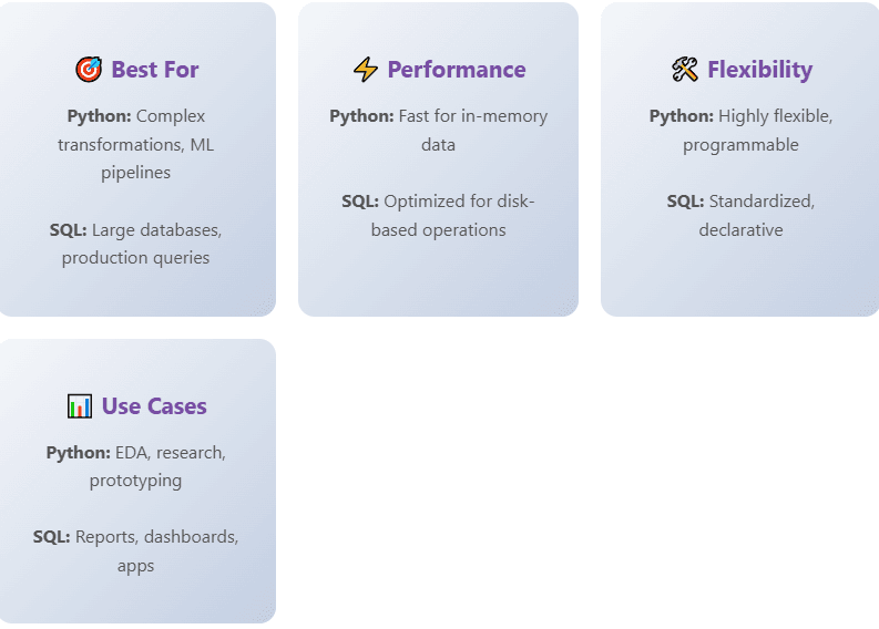
SQL window functions excel when your data already lives in a database and you need to perform analysis as part of a larger query workflow. If you’re building reports, dashboards, or application features that query databases directly, keeping calculations in SQL avoids data transfer overhead and leverages database optimization. Window functions are also excellent for one-off analytical queries where you want to explore data patterns without writing a full Python script.
For production systems serving multiple users, SQL’s transaction support and concurrent access handling make it a natural choice. The database can manage locks, ensure consistency, and optimize queries across multiple connections in ways that would be complex to replicate in application code.
When to Choose Pandas
Pandas becomes the better choice when you’re doing exploratory data analysis, building machine learning pipelines, or working with data from multiple sources that aren’t in a database. The flexibility to mix structured dataframe operations with arbitrary Python code enables rapid prototyping and complex transformations that would be awkward in SQL.
For datasets that fit in memory and workflows that involve multiple analysis steps, iteration, or statistical modeling, pandas provides a more productive environment. The ability to inspect intermediate results, visualize data at each step, and leverage Jupyter notebooks for reproducible analysis makes pandas ideal for research and development work.
Performance Comparison Table
| Operation Type | SQL Window Functions | Pandas GroupBy/Rolling | Best Choice |
|---|---|---|---|
| Simple aggregations on large database tables | Excellent | Good (with data transfer overhead) | SQL |
| Complex multi-step transformations | Good | Excellent | Pandas |
| Time-based rolling calculations | Good (vendor-dependent) | Excellent | Pandas |
| Ranking operations | Excellent | Excellent | Either |
| Operations on in-memory data | Good | Excellent | Pandas |
| Integration with other database operations | Excellent | Good | SQL |
What We’ve Seen
Throughout this exploration, we’ve discovered that SQL window functions and pandas group operations aren’t really competitors—they’re complementary tools designed for different contexts. SQL window functions provide a declarative, database-optimized approach that excels when data lives in a database and you need to perform analysis as part of query workflows. They offer excellent performance at scale, integrate seamlessly with database features, and provide a standardized way to express analytical calculations.
Pandas brings flexibility, a richer set of time series tools, and tight integration with Python’s data science ecosystem. It shines when you need to perform complex, multi-step transformations, work with data from multiple sources, or build end-to-end analytical pipelines that go beyond pure SQL capabilities.
The real question isn’t which is better, but which fits your specific workflow, infrastructure, and problem domain. Many data professionals find themselves using both: SQL for data extraction and initial aggregation where the data lives, and pandas for complex transformations and analysis in their application layer. Understanding the strengths of each approach allows you to make informed decisions about where to perform each operation in your data pipeline, ultimately leading to more efficient, maintainable, and performant solutions.
As data workflows become increasingly hybrid—spanning databases, data lakes, cloud services, and local computing environments—the ability to fluidly move between SQL and pandas operations becomes a valuable skill. Rather than viewing this as a debate with a winner, we should see it as an opportunity to leverage the right tool at the right time, building more robust and flexible data systems that can adapt to changing requirements and growing scale.