In the data engineering world, two titans compete for dominance in data transformation: SQL, the venerable language that has powered databases for nearly five decades, and Python with its pandas library, the modern darling of data scientists. The question isn’t which is better—it’s understanding when each shines and how to leverage both for maximum effectiveness.
Data transformation lies at the heart of every analytics pipeline. Whether you’re building ETL workflows, preparing datasets for machine learning, or generating business reports, the choice between SQL and Python shapes everything from development speed to performance at scale. According to recent industry analysis, this decision fundamentally determines how teams approach data engineering challenges in 2025.
The Fundamental Difference in Philosophy
SQL approaches data transformation declaratively. You describe what you want—filtered rows, aggregated values, joined tables—and the database engine determines how to execute it efficiently. This abstraction has powered enterprise data systems for decades, allowing databases to optimize queries automatically based on indexes, statistics, and execution plans.
Python’s pandas library takes an imperative approach. You specify explicit steps to transform DataFrames: filter this column, group by that field, apply these functions. This procedural nature provides granular control but shifts optimization responsibility from the database engine to the developer.
Deep Dive: For a comprehensive understanding of modern ETL practices, explore Airbyte’s detailed analysis of SQL vs Python in the AI era, which covers how both tools are evolving to handle AI-driven transformations.
Performance: Where Each Tool Excels
Performance comparisons between SQL and pandas reveal nuanced trade-offs that depend heavily on data size, operation type, and infrastructure configuration.
SQL’s Performance Strengths
SQL excels with large datasets that exceed memory capacity. According to performance benchmarks, SQL consistently outperforms pandas for basic operations like filtering, sorting, and aggregating on datasets with millions of rows. The reasons are fundamental to SQL’s architecture:
- Optimized storage: Binary formats with compression and efficient disk access patterns.
- Intelligent indexing: B-tree and hash indexes accelerate lookups and joins.
- Query optimization: Cost-based optimizers select efficient execution plans automatically.
- Parallel execution: Modern databases leverage multiple cores transparently.
-- SQL Example: Efficient Aggregation on Large Data
-- Execution time on 10M rows: ~3-5 seconds on standard DB infrastructure

SELECT
    customer_region,
    COUNT(*) as order_count,
    SUM(order_total) as revenue
FROM orders
WHERE order_date >= '2024-01-01'
GROUP BY customer_region
HAVING SUM(order_total) > 100000
ORDER BY revenue DESC;
Pandas’ Performance Sweet Spot
Pandas shines when data fits comfortably in memory and transformations involve complex logic that SQL handles awkwardly. DuckDB’s benchmarks demonstrate that for in-memory operations with sophisticated transformations, pandas can match or exceed SQL performance.
# Python/Pandas Example: Complex Transformation with Custom Logic
# Execution time on 1M rows: ~2-4 seconds
import pandas as pd
import numpy as np

# Assumes a CSV 'orders.csv' exists with 'total', 'customer_type', 'customer_id', 'region'
# Create dummy data for demonstration so the code runs:
data = {
    'order_id': range(1, 1001),
    'customer_id': np.random.randint(1, 100, 1000),
    'region': np.random.choice(['North', 'South', 'East', 'West'], 1000),
    'customer_type': np.random.choice(['B2B', 'B2C'], 1000),
    'total': np.random.uniform(100, 5000, 1000)
}
df = pd.DataFrame(data)

# --- Actual Transformation Logic ---

# Apply custom business logic row by row
df['discount_tier'] = df.apply(
    lambda row: 'premium' if row['total'] > 1000 and row['customer_type'] == 'B2B' else 'standard',
    axis=1
)

# Windowing operation: Calculate rolling average per customer
df['rolling_avg'] = df.groupby('customer_id')['total'].transform(
    lambda x: x.rolling(window=7, min_periods=1).mean()
)

# Final aggregation based on the new features
result = df.groupby(['region', 'discount_tier']).agg({
    'order_id': 'count',
    'total': ['sum', 'mean'],
    'rolling_avg': 'mean'
}).reset_index()

print(result.head())
The Memory Constraint Reality
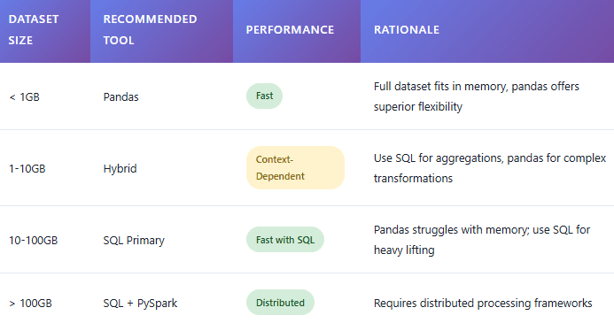
Pandas requires loading entire datasets into RAM. A developer’s laptop with 16GB might handle datasets up to 4-5GB comfortably, accounting for overhead and transformations. SQL databases operate differently—they stream results and use disk-based algorithms when queries exceed memory, enabling operations on terabyte-scale datasets that would crash pandas immediately. As data engineering practitioners note, this fundamental architectural difference drives many tool selection decisions.
The Data Size Decision Matrix
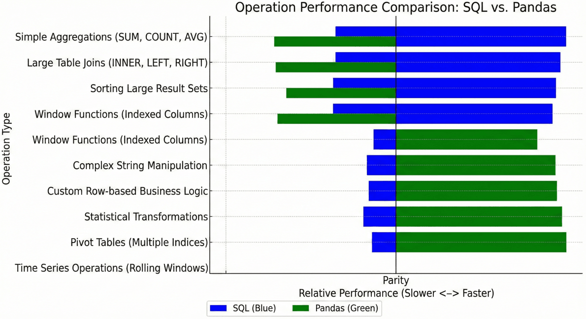
Operation-Specific Performance
Different operations favor different tools. Real-world benchmarks from Carwow’s engineering team reveal that the winner depends on the specific transformation:

Development Experience and Productivity
Performance isn’t everything. Developer productivity and code maintainability matter enormously in real projects.
SQL’s Clarity for Set Operations
SQL excels at expressing set-based operations clearly. Joins, unions, and aggregations map naturally to SQL’s declarative syntax. Anyone familiar with databases can read and understand a well-written SQL query without deep technical knowledge.
The Nested Query Problem: SQL’s readability deteriorates quickly with complex nested subqueries. What starts as elegant declarative code becomes an unreadable mess of parentheses and indentation. Common Table Expressions (CTEs) help, but complex data pipelines with multiple transformation stages often feel forced in pure SQL.
Pandas’ Iterative Development Flow
Pandas provides an interactive development experience that SQL struggles to match. In Jupyter notebooks or iPython, data scientists can execute transformations line-by-line, inspecting intermediate results at each step. This iterative workflow accelerates development and debugging significantly.
# Pandas Interactive Workflow Example
import pandas as pd
import numpy as np
# 1. Load data (Creating dummy data for this example)
df = pd.DataFrame({
'revenue': np.random.uniform(-100, 1000, 100),
'cost': np.random.uniform(10, 500, 100),
'signup_date': pd.date_range(start='2023-01-01', periods=100)
})
# 2. Inspect first rows (common interactive step)
# print(df.head())
# 3. Apply transformation Step 1: Filter
df_clean = df[df['revenue'] > 0].copy()
# 4. Check statistics of intermediate step
# print(df_clean.describe())
# 5. Create new features Step 2: Calculate margin
df_clean['margin_pct'] = (df_clean['revenue'] - df_clean['cost']) / df_clean['revenue']
# 6. Visualize distribution (in a notebook environment)
# df_clean['margin_pct'].hist()
print("Transformation complete. Head of cleaned data:")
print(df_clean.head())
According to data scientists discussing tool preferences, this step-by-step development pattern is why pandas proves more productive for exploratory data analysis and prototyping complex transformations.
The Hybrid Approach: Best of Both Worlds
Modern data engineering increasingly adopts hybrid architectures that leverage each tool's strengths. Leading ETL tools in 2025 enable seamless integration between SQL and Python.
Pattern 1: SQL for Extraction and Aggregation, Pandas for Complex Logic
This pattern uses the database to reduce the data size before loading it into memory for Python-specific operations like advanced statistical modeling or machine learning preparation.
import pandas as pd
import sqlalchemy as sa
from sklearn.preprocessing import StandardScaler
import numpy as np
# --- Setup dummy SQLite DB for this example to be "working" ---
# In a real scenario, replace this with your actual DB connection string
# e.g., 'postgresql://user:password@host:port/database'
engine = sa.create_engine('sqlite:///:memory:')
# Create some dummy data in the SQL DB
dummy_sales_data = pd.DataFrame({
'customer_id': np.random.randint(1, 50, 200),
'order_date': pd.date_range(start='2024-01-01', periods=200),
'product_category': np.random.choice(['A', 'B', 'C'], 200),
'quantity': np.random.randint(1, 10, 200),
'revenue': np.random.uniform(100, 1000, 200)
})
dummy_sales_data.to_sql('sales', engine, index=False)
# ---------------------------------------------------------
# 1. SQL handles the heavy lifting (Aggregation)
query = """
SELECT
customer_id,
product_category,
SUM(quantity) as total_quantity,
SUM(revenue) as total_revenue
FROM sales
WHERE order_date >= '2024-01-01'
GROUP BY customer_id, product_category
"""
# 2. Load aggregated data into pandas
df = pd.read_sql(query, engine)
# 3. Pandas handles complex transformations & Feature Engineering
df['revenue_per_unit'] = df['total_revenue'] / df['total_quantity']
# Complex binning based on customer total revenue
df['customer_segment'] = pd.cut(
df.groupby('customer_id')['total_revenue'].transform('sum'),
bins=[-np.inf, 5000, 15000, np.inf],
labels=['low', 'medium', 'high']
)
# 4. Apply ML utility from sklearn
scaler = StandardScaler()
# Ensure data is 2D for scalar
df['normalized_revenue'] = scaler.fit_transform(df[['total_revenue']])
print("Hybrid Transformation Result:")
print(df.head())
# 5. (Optional) Load results back to database
# df.to_sql('customer_analytics', engine, if_exists='replace', index=False)
Pattern 2: DuckDB - SQL Performance with Pandas Integration
DuckDB represents a game-changing approach: it runs SQL queries directly on pandas DataFrames with near-zero data transfer overhead. This enables developers to use SQL's optimization for operations where it excels while staying in the Python ecosystem.
import duckdb
import pandas as pd
import numpy as np
# Create dummy pandas DataFrames (representing data loaded from CSVs)
orders_data = {
'order_id': range(1, 101),
'customer_id': np.random.randint(1, 20, 100),
'total': np.random.uniform(50, 500, 100),
'order_date': pd.date_range(start='2024-01-01', periods=100)
}
customers_data = {
'customer_id': range(1, 21),
'customer_name': [f'Customer {i}' for i in range(1, 21)],
'customer_tier': np.random.choice(['Gold', 'Silver'], 20)
}
orders_df = pd.DataFrame(orders_data)
customers_df = pd.DataFrame(customers_data)
# --- Query pandas DataFrames directly with SQL using DuckDB ---
result_df = duckdb.sql("""
SELECT
c.customer_name,
c.customer_tier,
COUNT(o.order_id) as order_count,
SUM(o.total) as lifetime_value
FROM orders_df o
JOIN customers_df c ON o.customer_id = c.customer_id
WHERE o.order_date >= '2024-01-01'
GROUP BY c.customer_name, c.customer_tier
HAVING SUM(o.total) > 500 -- Lowered threshold for this small dummy dataset
""").df()
# Result is a pandas DataFrame ready for further processing
result_df['avg_order_value'] = result_df['lifetime_value'] / result_df['order_count']
print("DuckDB SQL on Pandas Result:")
print(result_df.head())
Real-World ETL Architectures
Modern ETL pipelines combine multiple tools strategically. Let's examine how organizations structure data transformation workflows.
The Modern Data Stack Approach (ELT)
The rise of ELT (Extract-Load-Transform) over traditional ETL reflects SQL's dominance in data warehouses. Tools like dbt (data build tool) enable teams to perform transformations entirely in SQL within data warehouses like Snowflake, BigQuery, or Redshift.
- Extract: Ingestion tools (Fivetran, Airbyte) move raw data to warehouses
- Load: Raw data lands in staging tables
- Transform: dbt orchestrates SQL transformations in the warehouse
- Consumption: BI tools query final tables, ML engineers extract to pandas
According to 2025 ETL tool surveys, this pattern has become the de facto standard for analytics engineering, with SQL handling 80-90% of transformation logic.
Python-First Data Science Workflows
Data science teams often adopt Python-centric pipelines where pandas, NumPy, and scikit-learn form the core. SQL becomes the interface to data sources rather than the primary transformation engine.
# Python-Centric ML Pipeline Sketch
import pandas as pd
from sklearn.ensemble import RandomForestClassifier
import numpy as np
from datetime import datetime

# --- Mocking the Database Interaction for this example ---
# In reality, use sqlalchemy connection as shown in Pattern 1
# df = pd.read_sql("SELECT * FROM analytics.customer_features", engine)

# Create dummy data representing the result of a DB query
df = pd.DataFrame({
    'customer_id': range(1, 101),
    'signup_date': pd.date_range(start='2023-01-01', periods=100),
    'feature_usage_count': np.random.randint(0, 100, 100),
    'categorical_segment': np.random.choice(['A', 'B'], 100),
    'target_churn': np.random.randint(0, 2, 100)
})
# ---------------------------------------------------------


# 1. Transform: Heavy pandas preprocessing
# Handle missing values (simulated)
df.loc[0:5, 'feature_usage_count'] = np.nan
df = df.dropna(subset=['feature_usage_count'])

# Feature engineering with datetime objects
current_date = datetime(2024, 1, 1)
df['days_since_signup'] = (current_date - df['signup_date']).dt.days

# One-hot encoding
df = pd.get_dummies(df, columns=['categorical_segment'], drop_first=True)

# Define features and target
feature_cols = ['feature_usage_count', 'days_since_signup'] + [col for col in df if col.startswith('categorical_segment_')]
X = df[feature_cols]
y = df['target_churn']

# 2. Train model
model = RandomForestClassifier(n_estimators=10, random_state=42)
model.fit(X, y)

# 3. Generate Predictions
predictions = pd.DataFrame({
    'customer_id': df['customer_id'],
    'predicted_churn_probability': model.predict_proba(X)[:, 1]
})

print("Predictions ready for DB upload:")
print(predictions.head())

# 4. Load predictions back to warehouse
# predictions.to_sql('ml_predictions', engine, if_exists='replace')
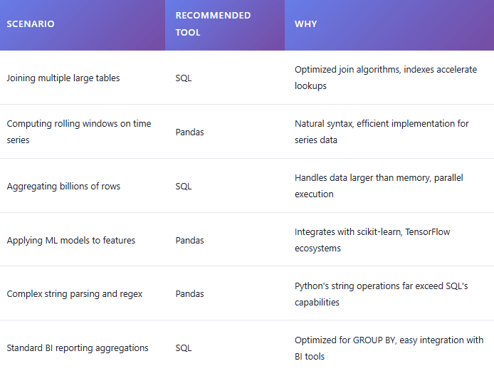
When to Choose What: Decision Framework
Conclusion
The narrative of "SQL vs. Python" is rapidly becoming obsolete in modern data engineering. As we move through 2025, framing data transformation as a zero-sum game between these two titans is a mistake that limits architectural potential. Instead of a competition, the landscape has shifted toward a pragmatic symbiosis.
SQL remains the undisputed foundation for scalable, set-based operations on massive datasets that exceed memory limits. Its declarative nature allows database engines to optimize heavy lifting far better than manual coding ever could. Conversely, Python and pandas provide the necessary surgical precision for complex procedural logic, iterative data exploration, and seamless integration with the machine learning ecosystem.
The most effective data architectures today are inherently hybrid. They don't force a choice; they leverage the strengths of both. Whether through ELT patterns using dbt, Python-centric ML pipelines that offload aggregation to the warehouse, or bridging technologies like DuckDB, the goal is to move processing to where it is most efficient.
Ultimately, the mark of an advanced data professional isn't deep allegiance to a single tool syntax. It is the architectural judgment to discern which approach offers the best combination of performance, maintainability, and development speed for the specific challenge at hand. The debate isn't about picking a winner; it's about mastering the convergence.