Why is the wave function continuous and differentiable?

In undergraduate quantum mechanics lectures, we are often taught that the wave function is continuous and differentiable. However, since few people seem to properly understand the reason for this, I would like to write a little about it.

From the standpoint of physics as an empirical science, if asked whether the actual wave function is differentiable even in the micro-region of the Planck length (about 10 to the power of -35 meters), the accurate answer is that it has not yet been verified by experiments.

Also, theoretically, there is doubt that position coordinates are continuous. If they are truly continuous, one must present a measurement method to prove it. Let us assume that position coordinates are continuous variables and consider how to measure the position of a particle in a region smaller than the Planck length. Generally, if one wants to build a measuring instrument with sensitivity to an extremely narrow spatial region, the quantum fluctuation of its position, Δx, must be made extremely small. From the uncertainty relation, this requires a very large quantum fluctuation of momentum, Δp, and the large energy fluctuation ΔE that it brings. If one tries to measure the position of that region while injecting such large energy fluctuations into a narrow area, the possibility of a mini black hole forming at that location increases. Even though one tried to measure the position of a point particle, the black hole created by the measuring device hides that position, making it impossible to measure. In other words, the measurement of position coordinates below the Planck length remains a conceptually unsolved problem.

If we consider a one-dimensional potential problem of the delta function type, the differential coefficient of the wave function differs on the left and right at that point, and it is not differentiable. However, in actual experiments, such potentials can only be created approximately, and in those real systems, the experimental results can be explained by a wave function that is continuous and also first-order differentiable.

The reason why non-differentiable wave functions do not appear in ordinary experiments is simply due to the energy cost of creating such a state. Since a non-differentiable wave function generally leads to higher momentum energy, it is just experimentally difficult to prepare that energy in advance.

For example, when finding the bound state of a potential problem, the condition that the energy eigenvalue of that state is finite is already required as a matter of physics, so non-differentiable wave functions where kinetic energy would diverge are excluded from the beginning.

It is also a problem that physics students who view quantum mechanics as mathematics impose completeness on an infinite-dimensional continuous state space without thinking about physics at all. Completeness is not a fact required by experiments as an empirical science. It is merely a model that is mathematically elegant and allows for various proofs to be made easily. For example, when effects up to quantum gravity are incorporated, there is no guarantee that nature follows that continuous complete model.

Even if particle system models such as harmonic oscillators are defined using a finite-dimensional state space, they are all consistent with experimental results to date. Therefore, theories without completeness or continuity have not been refuted by experiments.

In this textbook as well, we explain the particle position operator and momentum operator in Chapter 8, but those operators can be defined without taking the dimension N of the state space to infinity. And if N is sufficiently large, the harmonic oscillator in Chapter 9 can also be described by that finite-dimensional matrix, and it does not contradict all experimental results to date. Even if N is finite, the Heisenberg equation for the harmonic oscillator is properly satisfied. However, space is discretized. But for a sufficiently large N, the spatial interval can be made smaller than the Planck length, where quantum gravity is thought to begin to take effect. As long as space remains discrete, there is no problem with current physical theory, where experiments have not yet reached the Planck length region.

Let us think about this concretely. In a state space where N is finite, let us consider the following N basis vectors.

And with this basis, we define the following N-dimensional square matrix. This serves as an annihilation operator (lowering operator) for these basis vectors.

And the creation operator (raising operator) is defined by the Hermitian conjugate.

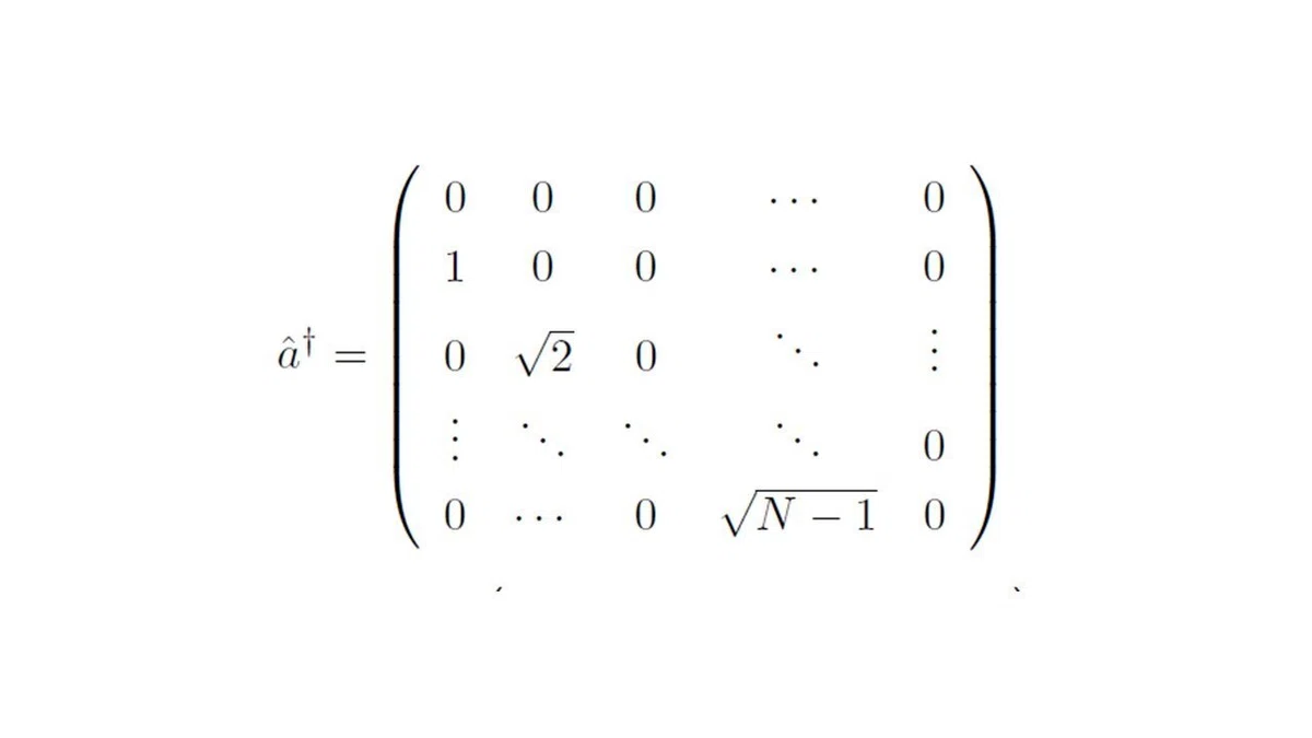
For example, each basis vector can be obtained by repeatedly applying the creation operator to the first vector and performing appropriate normalization.

Note that the commutation relation between the annihilation operator and the creation operator is slightly off in the finite-dimensional case, and it is not proportional to the identity matrix as it is. However, one can still create models such as harmonic oscillators in discrete space.

To create a harmonic oscillator model in discrete space, one can do so by defining a number operator as follows.

You can easily check that the basis vectors considered at the beginning are eigenvectors of this number operator.

Even in this finite-dimensional quantum mechanics, if we introduce a constant L with units of length and the Planck constant, we can introduce position and momentum operators (for discrete space) as follows.

However, unlike the continuous space case, the commutation relation between the position operator and the momentum operator is not yet exactly proportional to the identity operator I.

The eigenvalues and eigenvectors of the position operator when N is finite can be considered as follows. The same applies to the eigenvalues and eigenvectors of the momentum operator.

The reason we can create a harmonic oscillator model even in discrete space is that the commutation relations of the number operator and the creation operator are the same as in continuous space, as shown below.

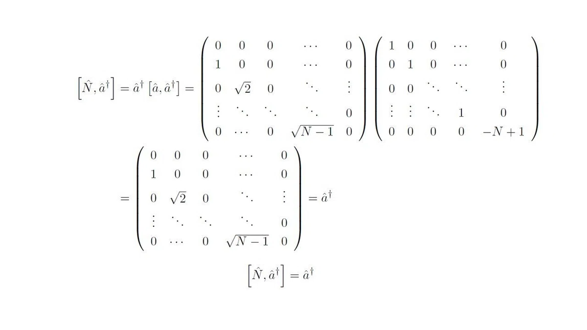
Incidentally, the commutation relation of the annihilation operator is also the same as in the case of continuous space.

Therefore, let us construct a Hamiltonian using a constant ω with units of angular frequency and the number operator, and consider time evolution using the unitary matrix below.

If we define the Heisenberg operators for the position operator and momentum operator using this operator, we can confirm that they exhibit the same motion as a classical harmonic oscillator, even in discrete space.

Here, we introduce the mass of this harmonic oscillator as follows.

Then, the form of the Heisenberg equations for position and momentum matches exactly the form of the classical equations of motion for a harmonic oscillator.

Therefore, the expectation values of position and momentum also satisfy the same equations as the classical equations of motion. This is the same as the classical harmonic oscillator equation that appears in Ehrenfest's theorem.

If you want to make the space continuous, you only need to consider quantum states that have low energy compared to ℏωN and take N to infinity. This causes the quantum harmonic oscillator model in continuous space to emerge.

Since the theory of the ordinary quantum harmonic oscillator in continuous space can be constructed through this line of reasoning as well, there are actually no subjects in physics that require worrying about rigorous mathematics. It is by no means the case that one cannot understand even the quantum mechanics of a harmonic oscillator without knowledge of mathematically rigorous functional analysis.