Consumer Theory (7): Slutsky Equation

We will organize the relationship between the utility maximization problem and the expenditure minimization problem discussed so far, and consider the most important theme in consumer theory: 'how does the demand for goods react to changes in market prices?' The series can be found here.

Duality of Consumption

When a consumer achieves a consumption plan $${x}$$ under a budget $${I}$$ and obtains utility $${u}$$, the consumer can view this as either 'having chosen a consumption that realizes maximum utility under a budget constraint (utility maximization)' or 'having chosen a consumption that results in the minimum budget among those that achieve the target utility (expenditure minimization).' This is called duality of consumption, and the actual consumption achieved at the optimal solution is equal to both the Walrasian demand and the compensated demand.

The utility function $${{u(x)}}$$ represents a continuous and locally non-satiated preference relation $${{\succsim}}$$. This preference relation $${{\succsim}}$$ is defined on the consumption set $${{X}}$$. Assume that the prices of $${{N}}$$ types of goods $${{p_i (i=1, \cdots, N)}}$$ are all positive real numbers. To prove duality, it suffices to show that the following (1) and (2) hold.

(1) If $${{x^* \in X}}$$ is a solution to the utility maximization problem with income $${{I}}$$, then $${{x^*}}$$ is a solution to the expenditure minimization problem with target utility $${{u(x^*)}}$$, and the minimum expenditure at this time is equal to $${{I}}$$.

(2) If $${{\bar x \in X}}$$ is a solution to the expenditure minimization problem with target utility level $${{u}}$$, then $${{\bar x}}$$ is a solution to the utility maximization problem with income $${{I=p\cdot x}}$$, and the maximum utility at this time is equal to $${{u}}$$.

Proof of (1)
We show by contradiction that '$${{x^*}}$$ is a solution to $${{\underset{x}{\max} u(x)　\text{s.t}. p\cdot x = I}}$$ $\Rightarrow$ $${{x^*}}$$ is a solution to $${{\underset{x}{\min} p\cdot x　\text{s.t}. u(x)=u(x^*)}}$$'.

Assuming $${{x^*}}$$ is not a solution to $${{\underset{x}{\min} p\cdot x　\text{s.t}. u(x)=u(x^*)}}$$, by the extreme value theorem, this expenditure minimization problem has a solution $${{x'\neq x^*}}$$.
At this time, $${{u(x')\geq u(x^*)}}$$ and $${{p \cdot x' < p \cdot x^* = I}}$$ hold. This is because the utility at solution $${{x'}}$$ is greater than the target utility $${{u(x^*)}}$$, and by the assumption of contradiction, the expenditure at solution $${{x'}}$$ is strictly smaller than $${{p \cdot x^*}}$$ since $${{x'\neq x^*}}$$.
Here, due to the local non-satiation of the preferences represented by $${{u(x)}}$$, we can find an $${{x''}}$$ arbitrarily close to $${{x'}}$$ such that $${{u(x'')>u(x')}}$$ and $${{p\cdot x'' < I}}$$. This implies $${{u(x'') > u(x^*)}}$$ and $${{p\cdot x'' < I}}$$, which contradicts the fact that $${{x^*}}$$ is a solution to the utility maximization problem. Therefore, the assumption is negated, and $${{x^*}}$$ is a solution to the expenditure minimization problem. Also, since $${{x^*}}$$ is a solution to the utility maximization problem, $${{p\cdot x^* = I}}$$.

* Even if the condition for the utility maximization problem is $${{p\cdot x^* \leq I}}$$, in a utility maximization problem under a continuous utility function $${{u(x)}}$$ representing preferences that satisfy local non-satiation, it can be said that $${{p\cdot x^* = I}}$$ because the solution $${{x^*}}$$ exists on the budget line according to Walras' Law.

Proof of (2)
We show by contradiction that '$${{x^*}}$$ is a solution to $${{\underset{x}{\min} p\cdot x　\text{s.t}. u(x) = u (>u(0))}}$$ $\Rightarrow$ $${{x^*}}$$ is a solution to $${{\underset{x}{\max} u(x)　\text{s.t}. p\cdot x = I}}$$'.

Assuming $${{x^*}}$$ is not a solution to $${{\underset{x}{\max} u(x)　\text{s.t}. p\cdot x = I}}$$, by the extreme value theorem, this utility maximization problem has a solution $${{x'\neq x^*}}$$.
At this time, $${{u(x')>u(x^*)}}$$ and $${{p \cdot x' \leq p \cdot x^* = I}}$$ hold. By the assumption of contradiction, the utility at solution $${{x'}}$$ is strictly greater than $${{u(x^*)}}$$ since $${{x'\neq x^*}}$$. $${{x'}}$$ is a point within the budget.
Here, due to the continuity of $${{u(x)}}$$, considering $${{x''=\alpha x'}}$$ where $${{\alpha \in (0, 1)}}$$, as $${{\alpha \to 1}}$$, from the density of $${{u(x)}}$$, there exists a $${{c}}$$ such that $${{u(x')>c>u(x^*)}}$$, and since we can consider an $${{\alpha}}$$ such that $${{c=u(x'')}}$$, at this time $${{u(x'')>u(x^*)}}$$ holds. Also, when $${{x''=\alpha x'<x'}}$$, since each component of the price vector is a positive real number, $${{p\cdot x'' < p\cdot x'}}$$ holds. Therefore, from $${{p\cdot x'' < p\cdot x'\leq p \cdot x^* }}$$, we get $${{p\cdot x'' < p \cdot x^* }}$$. This contradicts the fact that $${{x^*}}$$ is a solution to the expenditure minimization problem. Therefore, the assumption is negated, and $${{x^*}}$$ is a solution to the utility maximization problem. Furthermore, from the property of non-excess utility in compensated demand, the maximum utility at that time is equal to $${{u}}$$.

Slutsky Equation

The most important theme in consumer theory is to understand how demand, which is the aggregate of rational consumer behavior, reacts to changes in market prices, that is, to formulate the change in Walrasian demand due to price fluctuations $${{\dfrac{\partial x_i(p, I)}{\partial p_j}}}$$.

From the duality of the utility maximization problem and the expenditure minimization problem, $${{\bar x_i(p, u) = x_i(p, I(p, u))}}$$ holds. Differentiating both sides with respect to the price of the $${{j}}$$-th good, by the chain rule,

$${{\dfrac{\partial \bar x_i(p, u)}{\partial p_j}=\dfrac{\partial x_i(p, I(p, u))}{\partial p_j}+\dfrac{\partial x_i(p, I(p, u))}{\partial I(p, u)}\dfrac{I(p, u)}{\partial p_j}}}$$

holds. By using Shephard's Lemma $${{\dfrac{I(p, u)}{\partial p_j}=\bar xj}}$$ and the duality relationship $${{\bar x_i(p, u) = x_i(p, I(p, u))}}$$ to organize, we obtain the following Slutsky equation.

Thus, the relationship between the rational consumer behaviors discussed so far: the utility maximization problem and the expenditure minimization problem, is organized as follows.

The derivation of the Slutsky equation itself is within the scope of our previous discussions using Shephard's Lemma, the chain rule of differentiation, and the duality of consumption, and it is not particularly difficult. What is more important for understanding the Slutsky equation is to clarify what this equation means economically. In conclusion, it means that "the change in demand due to price fluctuations $${\dfrac{\partial x_i(p, I)}{\partial p_j}}$$ is equal to the sum of the substitution effect$${\dfrac{\partial \bar x_i(p, u)}{\partial p_j}}$$ and the income effect$${-\dfrac{\partial x_i(p, I)}{\partial I} x_j(p, I)}$$.

Substitution Effect and Income Effect

Substitution Effect

Last time, we derived the Law of Compensated Demand from the properties of the compensated demand $${\bar x(p, u)}$$, which is the solution to the expenditure minimization problem, and defined the own-substitution effect within it.

The substitution effect represents the change in the consumption quantity (= compensated demand quantity) of a certain good or another good when the price of a certain good changes, while keeping the target utility level constant. As mentioned above, when the price of a certain good rises, the compensated demand for that good itself does not increase (the own-substitution effect is non-positive). In the case of two or more goods, substitutability is defined by the change in the compensated demand quantity of another good accompanying a price change of a certain good, $${\dfrac{\partial \bar x_i(p, u)}{\partial p_j}}$$, which is called the
cross-substitution effect. Especially in the case of two goods, it graphically represents the curvature of the indifference curve. The more curved the indifference curve is, the less the compensated demand quantity changes with respect to price changes (= substitutability is small, and complementarity is large), and conversely, the flatter the indifference curve is, the more the compensated demand quantity changes with respect to price changes (= substitutability is large, and complementarity is small). The figure below shows the curvature of the indifference curve and the substitutability/complementarity of two goods, and the perfect substitutes and perfect complements introduced in the 3rd session are extreme examples of this.

For example, when the utility function of a two-good model is given by $${u(x_1, x_2)=x_1^ax_2^{1-a},  a\in (0,1)}$$, solving the expenditure minimization problem $${\underset{x}{\min}   p\cdot x　\text{s.t}.   u(x)=u}$$ using the Lagrange multiplier method yields,

$${\bar x_1=\Bigg(\dfrac{a}{1-a}\dfrac{p_2}{p_1} \Bigg)^{1-a}u}$$ and $${\bar x_2=\Bigg(\dfrac{1-a}{a}\dfrac{p_1}{p_2} \Bigg)^{a}u}$$

and differentiating these with respect to $${p_1}$$ and $${p_2}$$ respectively gives

$${\dfrac{\partial \bar x_1}{\partial p_1}=-\dfrac{1-a}{p_1}\Bigg(\dfrac{a}{1-a}\dfrac{p_2}{p_1}\Bigg)^{1-a}u≤0}$$ and $${\dfrac{\partial \bar x_1}{\partial p_2}=\dfrac{a}{p_1}\Bigg(\dfrac{1-a}{a}\dfrac{p_1}{p_2}\Bigg)^{a}u≥0}$$

$${\dfrac{\partial \bar x_2}{\partial p_1}=\dfrac{1-a}{p_2}\Bigg(\dfrac{a}{1-a}\dfrac{p_2}{p_1}\Bigg)^{1-a}u≥0}$$ and $${\dfrac{\partial \bar x_2}{\partial p_2}=-\dfrac{a}{p_2}\Bigg(\dfrac{1-a}{a}\dfrac{p_1}{p_2}\Bigg)^{a}u≤0}$$

from which we can see that the own-substitution effects $${\dfrac{\partial \bar x_1}{\partial p_1}}$$ and $${\dfrac{\partial \bar x_2}{\partial p_2}}$$ are non-positive.

Also, due to the symmetry of the utility function, the cross-substitution effect is $${\dfrac{\partial \bar x_1}{\partial p_2}=\dfrac{\partial \bar x_2}{\partial p_1}}$$ and is non-negative. Note that from the conditions of expenditure minimization, the cross-substitution effect in a two-good model is always non-negative (the non-positivity of the own-substitution effect holds generally, not just in the two-good model).

When there are many goods, substitutability and complementarity are defined by the sign of $${\dfrac{\partial \bar x_i(p, u)}{\partial p_j}}$$ as follows.

As an example, consider the compensated demand for Good 1: white rice, Good 2: furikake (rice seasoning), and Good 3: bread. When the price of white rice rises, if the compensated demand for white rice falls, the compensated demand for other goods must be changed to maintain the utility level. In this case, if the consumption of furikake decreases along with white rice $${\bigg(\dfrac{\partial x_2}{\partial p_1}\bigg)<0}$$, while the consumption of bread increases $${\bigg(\dfrac{\partial x_3}{\partial p_1}\bigg)>0}$$, then furikake is a complementary good and bread is a substitute good. Note that complementary goods are more generally defined as "goods that change in the same direction as the compensated demand for the $${i}$$-th good when the price of the $${i}$$-th good changes," so if we define a good $${j}$$ as a complementary good when $${\dfrac{\partial \bar x_i(p, u)}{\partial p_j}=0}$$ given $${\dfrac{\partial \bar x_i(p, u)}{\partial p_i}=0}$$, we can define complementary goods including the two-good case in the equality case.

Income Effect

When the price $${p_i}$$ of the $${i}$$-th good increases by $${Δp_i>0}$$, consider the additional expenditure required to maintain the same utility $${u}$$ as before the price increase. From Shephard's Lemma and the duality of consumption, $${∂I(p, u)/∂p_i=x_i}$$ holds. Here, for a small change in price $${Δp_i}$$, $${ΔI ≈ x_iΔp_i}$$ holds approximately. In other words, it represents the effect of a reduction in real income by $${x_iΔp_i}$$ due to the price increase of the good." On the other hand, one might consider the possibility that by reducing the consumption $${x_i}$$ of the good whose price has increased and increasing the consumption of other goods, utility could be further improved, making the additional expenditure required to maintain the target utility $${u}$$ less than $${ΔI}$$; however, the above equation indicates that in the limit of $${p_i→0}$$, this additional effect is negligible. The term $${-∂x_i(p, I)/∂I · x_iΔp_i}$$, obtained by multiplying the real change in income due to this price increase, $${x_iΔp_i}$$, by the coefficient $${-∂x_i(p, I)/∂I}$$, is called the income effect.

Note that while $${∂x_i(p, I)/∂I}$$ alone is sometimes referred to as the income effect, this is because this coefficient defines normal goods, neutral goods, and inferior goods as discussed in the fifth lecture.

Among inferior goods, those that satisfy $${|∂ar{x}_i(p, u)/∂p_j| < |∂x_i(p, I)/∂I · x_j|}$$ are called Giffen goods." Considering the case where $${i=j}$$ in the Slutsky equation,

$${∂x_i(p, I)/∂p_i = ∂ar{x}_i(p, u)/∂p_i - ∂x_i(p, I)/∂I · x_i(p, I)}$$

The first term on the right side is less than or equal to zero due to the own-substitution effect, and the second term on the right side is positive due to it being an inferior good; if the above condition is met, then $${∂x_i(p, I)/∂p_i > 0}$$, meaning it is theoretically possible to assume a good for which demand increases as the price increases. It is said that there are few cases where Giffen goods have been observed in reality.

Graphical interpretation of both effects

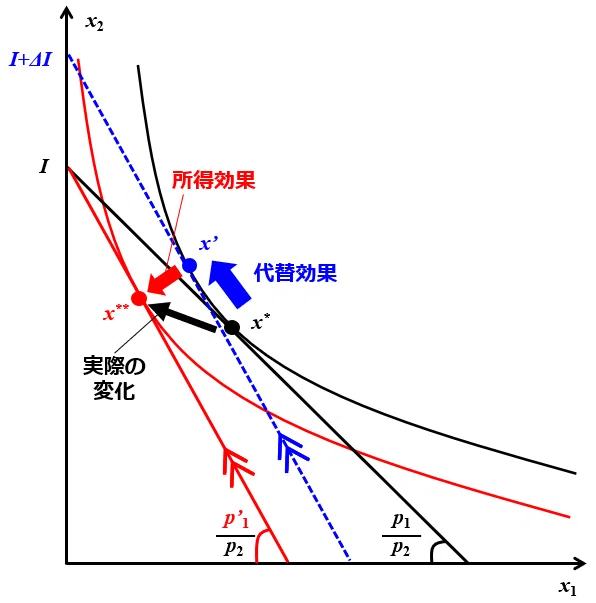
Regarding the effects of the substitution effect and income effect on consumption discussed so far, we attempt a graphical understanding using a two-good model. As shown in the figure below, consider the case where the optimal consumption plan moves from $${x^*→x^{**}}$$ as a result of an increase in the price $${p_1}$$ of the first good. According to the Slutsky equation, by introducing a hypothetical consumption plan $${x'}$$, this can be decomposed into Step 1: movement from $${x^*→x'}$$ and Step 2: movement from $${x'→x^{**}}$$.

Step 1 ($${x^*→x'}$$): Substitution effect and (hypothetical) subsidy
Because the budget line becomes steeper due to the increase in price $${p_1}$$, if the budget $${I}$$ is constant, utility must be lowered (movement from the black indifference curve to the red indifference curve in the figure). However, here we assume that a hypothetical subsidy is introduced, and that the initial utility level could be maintained even after the price increase occurred. Graphically, this means drawing a straight line that is parallel to the budget line that became steeper after the price increase and tangent to the initial indifference curve (the blue dashed budget line in the figure). At this time, the movement from $${x^*}$$ to the hypothetical optimal consumption plan $${x'}$$ represents the substitution effect, and the amount of subsidy additionally provided to maintain the utility level is the difference in the intercepts of the budget lines, $${ΔI}$$ is the amount.

Step 2 ($${x'→x^{**}}$$): Income effect
However, in reality, such a hypothetical subsidy does not exist, so the budget line shifts downward in parallel by the amount of the subsidy. This subsidy portion $${-ΔI}$$ is the effect where income decreases by the income effect, and the consumption after the decrease is the consumption $${x^{**}}$$ that is actually realized.

Price elasticity of demand

As an analysis example using the Slutsky equation, we take up the price elasticity of demand. The price elasticity of demand represents the ratio of the demand reduction rate (%) when the price increases by 1%, and is usually defined as follows as an indicator that is not affected by units.

Since sales are $${px(p)}$$, differentiating this with respect to price gives,

$${dpx(p)/dp = x + p · dx(p)/dp = x{1 - (-dx/dp · p/x)}}$$

We obtain this. Therefore, when $${(-dx/dp · p/x) < 1}$$, $${dpx(p)/dp > 0}$$, meaning that when the price elasticity is less than (or greater than) 1, raising the price increases (decreases) sales.

※ Examples of price elasticity of demand: Gas: 0.21, Beef: 0.94, Dining out: 1.3. Since the elasticity of gas is less than 1, demand does not decrease much even if the price is raised, and sales increase. Therefore, sales would be maximized by limiting the sales volume and raising the price. Since the elasticity of beef is almost 1, sales remain almost constant even if the price is changed. Since the elasticity of dining out is greater than 1, demand drops significantly when the price is raised, and sales decrease. Therefore, a strategy of low margins and high turnover by lowering the price would be effective.

Here, we further analyze price elasticity using the Slutsky equation. Considering the case where $${i=j}$$ in the Slutsky equation, we obtain the following equation.

$${∂x_i(p, I)/∂p_i = ∂ar{x}_i(p, u)/∂p_i - ∂x_i(p, I)/∂I · x_i(p, I)}$$

To express the left-hand side as an elasticity formula, multiply both sides by $${-\dfrac{p_i}{x_i}}$$ to obtain the following equation.

$${-\dfrac{\partial x_i}{\partial p_i}\dfrac{p_i}{x_i}=-\dfrac{\partial \bar x_i}{\partial p_i}\dfrac{p_i}{x_i}+\bigg(\dfrac{\partial x_i}{\partial I}\dfrac{I}{x_i}\bigg)\dfrac{p_ix_i}{I}}$$

Qualitatively, this equation can be decomposed and interpreted as follows.
(Price elasticity of demand) = -(Price elasticity of compensated demand) + (Income elasticity) × (Expenditure share)
Therefore, the conditions under which the price elasticity of demand increases can be summarized as follows.

• Close substitutes exist⇔ The price elasticity of compensated demand is high, and substitution to similar products occurs quickly due to price fluctuations

• The income elasticity of demand is high⇔ The rate of increase in demand when income increases by 1% is high
  * Goods with an income elasticity of demand greater than 1 are called luxury goods.

• The expenditure amount for that good accounts for a large share of income

In the examples above, the background of price elasticity can be qualitatively summarized as follows.
Gas has no close substitutes and is not a luxury good, so its income elasticity is not high, but it accounts for a certain share of income. Overall, its price elasticity is small.
Beef has close substitutes (pork, chicken, etc.) and is a luxury good, so its income elasticity is high. However, since its share of income is not large, its price elasticity is moderate.
Dining out has close substitutes (home cooking, takeout, etc.) and is a luxury good, so its income elasticity is high. Also, because it accounts for a large share of income, its price elasticity is high.

From next time, we will cover producer theory.