SYSTEM NOTICE

Auto translation by AI. Be sure, accuracy, nuances and authorial intent may not be fully reflected.

1-10 Laspeyres Index Formula: Calculating Fruit Price Indices

2023年4月1日 11:51

This statistical topic

We will calculate fruit price indices using the Laspeyres, Paasche, and Fisher formulas.
Are the trends in fruit prices and consumption being laid bare!?

Preparing the Official Problem Collection

We will use problems from the "Official Problem Collection." Please have the official problem collection ready.
If you do not have the official problem collection, do not worry!
Please enjoy statistics at your own pace in the "Learn" and "Practice" chapters!

Solving the problem

📘 Official Problem Collection Category

Field of univariate descriptive statistics
Question 10: Laspeyres Index Formula
(Annual purchase quantity and average price per household for pears and grapes)

Exam date
Statistics Certification Grade 2, November 2018, Question 4 (Answer Number 7)

Problem

Please refer to the official problem collection.

How to solve

The Laspeyres index is used for price indices (consumer price indices).
In the calculation of price × quantity, I will briefly state the characteristics of the Laspeyres index formula.

$$
\cfrac{Price in comparison year \times \boldsymbol{Quantity in base year}}{Price in base year \times \boldsymbol{Quantity in base year}} \times 100
$$

Fix the "Quantity in base year" (quantity in a specific year) and calculate the ratio of the comparison year to the base year in terms of price.
The key point is that the Laspeyres index is measured using the "Quantity in base year".

When dealing with multiple items, add the items to the denominator and numerator.
Next is an example with two items.

And let's pay attention to the following calculation formula.

The fraction on the left is the "monetary proportion of item 1 in the base year" for all items.
By multiplying by the fraction on the right, the "price ratio of item 1 between the comparison year and the base year," you can calculate the "monetary proportion of item 1 in the comparison year."

Since the fraction on the left is "base year data," once it is created for the base year, it can be used continuously for subsequent calculations.
In other words, "you can calculate the price index for the comparison year just by obtaining the price data for the comparison year in the future!"
This point is said to be the advantage of the Laspeyres index.

Returning to the problem.

Illustration of pears and grapes: From "Irasutoya"

In the Laspeyres index calculation formula for multiple items, replace item 1 with pears and item 2 with grapes.

The base year is 2016, and the comparison year is 2017.
Let's plug the specific values for the purchase quantity and average unit price of pears and grapes into the formula above.

The option corresponding to this formula is ②.
Note that the calculation result of this formula is $${104.864 \cdots}$$.

It appears that the price of pears + grapes has "risen by nearly 5% in one year".
Is the demand for pears and grapes strong?
Did the increase in demand for high-end varieties such as Shine Muscat boost the overall rise in sales prices?

Illustration of a fruit basket "Fruit in a basket": From "Irasutoya"

Answer

It is ②.

Difficulty: Easy

・Knowledge: Laspeyres index
・Calculation skills: Formula construction (low)
・Estimated time: 1 minute

Learn

Representative Price Indices

📕Official Textbook: 1.7.5 Creation and Use of Indices (from page 46)
Covers the Laspeyres index, Paasche index, and Fisher index.

I found a page on the Statistics Bureau of Japan's website that covers the Laspeyres formula, Paasche formula, and Fisher formula in the "Q&A (Answers) regarding the Consumer Price Index," so I would like to introduce it.

The "Consumer Price Index (CPI)," which is the parent page of this page, contained various information related to the Consumer Price Index.
If you are interested in price indices published by the government, please take a look.

Now, let's start calculating the "Price Index for Pears and Grapes"!

Laspeyres index
Fixes the quantity of the base year is an index that looks at price fluctuations.
You can calculate the price index for two items using the following formula.

Let's set Item 1 = Pears, Item 2 = Grapes, Base Year = 2020, and Comparison Year = 2021, and apply the data for pears and grapes.

$$
\begin{align*}
&\cfrac{Average price of pears in 2021 \times Purchase quantity in 2020 + Average price of grapes in 2021 \times Purchase quantity in 2020} {Average price of pears in 2020 \times Purchase quantity in 2020 + Average price of grapes in 2020 \times Purchase quantity in 2020} \times 100\\
&=\cfrac{66.26 \times 2497 + 149.62 \times 2262}{64.00 \times 2497 + 137.40 \times 2262} \times 100\\
&=107.07 \cdots
\end{align*}
$$

The Laspeyres index is 107.1.

■ Mathematical Expression
First, here is the mathematical expression for the two items above.
Let Item 1, 2 be $${i=1,2}$$, the base year be $${T=0}$$, and the comparison year be $${T=t}$$, and express price as $${p_{iT}}$$ ($${price_{item i, year}}$$) and quantity as $${q_{iT}}$$ ($${quantity_{item i, year}}$$).

$$
\cfrac{ p_{1t} \times q_{1\ 0} + p_{2t} \times q_{2\ 0} }
{ p_{1\ 0} \times q_{1\ 0} + p_{2\ 0} \times q_{2\ 0} } \times 100
$$

In preparation for cases with three or more items, we express it using Σ.
Let n items 1, 2, ..., n be $${i=1,2,\cdots , n}$$.
The base year price is $${p_{i0}}$$, the base year quantity is $${q_{i0}}$$, the comparison year price is $${p_{it}}$$, and the comparison year quantity is $${q_{it}}$$.
Also, since the denominator and numerator are calculated separately, we set the n items 1, 2, ..., n in the denominator as $${j=i,2,\cdots, n}$$.

$$
\begin{align*}
&Laspeyres index P_{\mathrm{L}(0, t)}\\
&=\cfrac{p_{1t} \times q_{1\ 0} + p_{2t} \times q_{2\ 0} + \cdots + p_{nt} \times q_{n0}}
{p_{1\ 0} \times q_{1\ 0} + p_{2\ 0} \times q_{2\ 0} + \cdots + p_{n0} \times q_{n0} } \times 100 \\
&=\cfrac{\displaystyle \sum^n_{i=1} p_{it}q_{i0}}{\displaystyle \sum^n_{j=1} p_{j0}q_{j0}} \times 100
\end{align*}
$$

Also, the official textbook uses the following formula to explain the Laspeyres index as a "weighted arithmetic mean using the base year composition ratio $${s_{i0}}$$ as the weight".

$$
Laspeyres index P_{\mathrm{L}(0, t)}=\sum s_{i0} \left(\cfrac{p_{it}}{p_{i0}} \right)\\
where s_{i0}=\cfrac{p_{i0}q_{i0}}{\sum_j p_{j0}q_{j0}}
$$

Raspberry illustration (fruit): From "Irasutoya"

Paasche index
An index that looks at price fluctuations by fixing the quantity of the comparison year.
You can calculate the price index for two items using the following formula.

Let Item 1 = Pears, Item 2 = Grapes, Base Year = 2020, and Comparison Year = 2021, and apply the data for pears and grapes.

$$
\begin{align*}
&\cfrac{Average price of pears in 2021 \times Purchase quantity in 2021 + Average price of grapes in 2021 \times Purchase quantity in 2021} {Average price of pears in 2020 \times Purchase quantity in 2021 + Average price of grapes in 2020 \times Purchase quantity in 2021} \times 100\\
&=\cfrac{66.26 \times 2617 + 149.62 \times 2127}{64.00 \times 2617 + 137.40 \times 2127}\times 100\\
&=106.94 \cdots
\end{align*}
$$

The Paasche index is 106.9.

$$
\cfrac{ "p_{1t} \times q_{1t}" + "p_{2t} \times q_{2t}" }
{ "p_{1\ 0} \times q_{1t}" + "p_{2\ 0} \times q_{2t}" } \times 100
$$

$$
\begin{align*}
&Paasche index P_{\mathrm{P}(0, t)}\\
&=\cfrac{p_{1t} \times q_{1t} + p_{2t} \times q_{2t} + \cdots + p_{nt} \times q_{nt}}{p_{1\ 0} \times q_{1t} + p_{2\ 0} \times q_{2t} + \cdots + p_{n0} \times q_{nt} } \times 100 \\
&=\cfrac{\displaystyle \sum^n_{i=1} p_{it}q_{it}}{\displaystyle \sum^n_{j=1} p_{j0}q_{jt}} \times 100
\end{align*}
$$

Also, the official textbook uses the following formula to explain the Paasche index as a "weighted harmonic mean using the comparison year composition ratio $${s_{it}}$$ as the weight".

$$
Paasche index P_{\mathrm{P}(0, t)}=\left( \sum s_{it} \left(\cfrac{p_{it}}{p_{i0}} \right)^{-1} \right)^{-1}\\
where s_{it}=\cfrac{p_{it}q_{it}}{\sum_j p_{jt}q_{jt}}
$$

Fisher Index
The Fisher index is the geometric mean of the Laspeyres index and the Paasche index.It is.

$$
\begin{align*}
&Fisher Index P_{\mathrm{F}(0, t)}\\
&=\sqrt{ Laspeyres Index P_{\mathrm{L}(0, t)} \times Paasche Index P_{\mathrm{P}(0, t)}}\\
\end{align*}
$$

Let's calculate.

$$
\sqrt{107.07 \cdots \times 106.94 \cdots}=107.00 \cdots
$$

The Fisher index is 107.0.

Illustration of a fisherman: From "Irasutoya"

The geometric mean is covered in the article "1-6 Calculation Formula for Average Rate of Change."
Please read this article as well if you like.

Practice

Let's try calculating the price index

"Annual purchase quantity and average price data per household" is published on the government statistics portal site "e-Stat."

This is statistical data included in the "Family Income and Expenditure Survey" by the Statistics Bureau of the Ministry of Internal Affairs and Communications.

You can download the EXCEL file from the page at the following link.
Family Income and Expenditure Survey / Income and Expenditure, Households of Two or More Persons, Annual Report

This is the "Annual expenditure, purchase quantity, and average price per item per household (households of two or more persons)" data for "Vegetables, Seaweed (Dried/Seaweed), Fruits," including pears and grapes.
It includes information such as trends from 2000 to 2021.

Download CSV file
You can download the formatted CSV file from this link.
This is the expenditure, purchase quantity, and average price data for fruit items from 2000 to 2021.
If you are using the Python sample file, please download this CSV file.

Let's try creating it with a calculator or by hand!

Let's practice the content of "Learn" by doing it by hand and calculating!
It is the most memorable method, and it also serves as training for calculator work during actual exams.

Let's try creating it in EXCEL!

When there is a large amount of data, doing it by hand becomes inefficient.
If you can learn to use a computer to create tables quickly, it will be easier to apply in practical work.

Calculating Price Index
It seems there is no dedicated function in Excel for calculating price indices.
As a topic, the 'GEOMEAN function' used for calculating the geometric mean of the Fisher index is relevant.
This is introduced in '1-6 Calculation Formula for Average Rate of Change'.

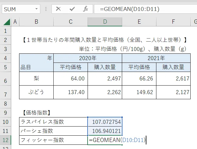
EXCEL: Example of using the GEOMEAN function

Calculating price indices for various years and fruits
I have included a price index simulator in the EXCEL sample file!
Though, it is a simple method.
By referencing raw data like this...

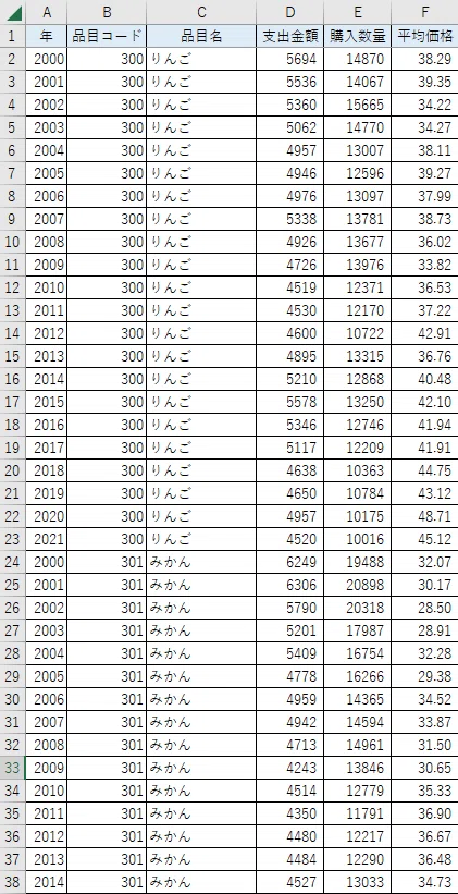
Calculate the price index on the simulator screen.
It seems the prices of apples and mandarin oranges have fallen from 2020 to 2021.

EXCEL: Example of using INDEX and MATCH functions

Changing the 'Year' and 'Item' in the red frame will also change the price index.
For example, let's change the combination to '2010' and '2021', and 'watermelon' and 'melon'.
It appears that the prices of watermelons and melons have risen by nearly 30% over 11 years.

Price index of watermelons and melons (2010-2021)

Try changing to various combinations of years and fruits included in the raw data to experience the fluctuations in the price index.
You might be able to see trends in fruit prices.
Please check it out for yourselves!

The sample file includes an 'Average Price Trend Graph'.

Downloading the EXCEL sample file
You can download the EXCEL sample file from this link.

Let's try creating it with Python!

Reading the program code, running the data, changing the data, and following the data is also an effective way to grasp the tabulation logic.
If you have sample code ready, you can automate similar tabulation tasks and get results quickly.

This time, let's work on calculating the price index for all fruits.
Also, since we have time-series data, let's plot a time-series graph.

1. Importing libraries

import pandas as pd
import numpy as np
import matplotlib.pyplot as plt
plt.rcParams['font.family'] = 'MS Gothic'
%matplotlib inline

2. Loading the CSV file
First, download the CSV file from the download link above.
Then, execute the following code to load the CSV file into a pandas DataFrame.

datafile = './sample_data.csv' # CSVファイルの格納フォルダとファイル名を設定
df = pd.read_csv(datafile)
print(df.shape)
display(df.head())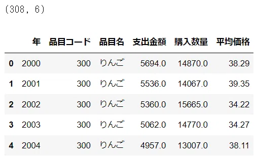

3. Calculating the price index
I could not find a dedicated function for calculating the price index.
Therefore, I will define a custom function that approximates the price index calculation formula.

■ Defining functions to make data easier to handle
Set the variables, etc., used in the price index calculation formula.

# 計算要素の取得関数
# データフレームから次の計算要素を取得する。
# n   : 品目数
# p_0 : 基準年の平均価格
# q_0 : 基準年の購入数量
# p_t : 比較年の平均価格
# q_t : 比較年の購入数量
def get_values(base_year, comp_year, df_data):      
    item_list = get_item_list(df_data)
    n = len(item_list)
    p_0 = df_data[df_data['年']==base_year]['平均価格'].reset_index(drop=True)
    q_0 = df_data[df_data['年']==base_year]['購入数量'].reset_index(drop=True)
    p_t = df_data[df_data['年']==comp_year]['平均価格'].reset_index(drop=True)
    q_t = df_data[df_data['年']==comp_year]['購入数量'].reset_index(drop=True)
    return n, p_0, q_0, p_t, q_t

# 品目リストの取得関数
def get_item_list(df_data):
    return df_data['品目名'].value_counts(sort=False).index.to_list()

■ Definition of three price index functions
・Laspeyres index: laspeyres_index
・Paasche index: paasche_index
・Fisher index: fisher_index
The arguments are the base year, comparison year, and the dataframe df.
Since the code would become long, I have extracted the denominator (denom) of the calculation formula.
Combining the code for the denominator calculation and the calculation for each index makes it resemble the mathematical formula.

# ラスパイレス指数関数
def laspeyres_index(base_year, comp_year, df_data):
    # 計算要素の取得
    n, p_0, q_0, p_t, q_t = get_values(base_year, comp_year, df_data)
    # 分母の計算
    denom =  sum([p_0[j] * q_0[j] for j in range(n)])
    # ラスパイレス指数の計算
    index_val = sum([p_t[i] * q_0[i] / denom for i in range(n)]) * 100
    return index_val

# パーシェ指数関数
def paasche_index(base_year, comp_year, df_data):
    # 計算要素の取得
    n, p_0, q_0, p_t, q_t = get_values(base_year, comp_year, df_data)
    # 分母の計算
    denom =  sum([p_0[j] * q_t[j] for j in range(n)])
    # パーシェ指数の計算    
    index_val = sum([p_t[i] * q_t[i] / denom for i in range(n)]) * 100
    return index_val

# フィッシャー指数関数
def fisher_index(base_year, comp_year, df_data):
    # ラスパイレス指数の計算
    l = laspeyres_index(base_year, comp_year, df_data)
    # パーシェ指数の計算
    p = paasche_index(base_year, comp_year, df_data)
    # フィッシャー指数の計算
    return np.sqrt(l * p)

■Calculation and display of the three price indices
Set the base year base_year and the comparison year comp_year.
Please try setting various years and checking the index calculation results..

# 設定 基準年と比較年を指定する
base_year = 2020  # 基準年
comp_year = 2021  # 比較年

# 指数の計算
laspeyres = laspeyres_index(base_year, comp_year, df)
paasche = paasche_index(base_year, comp_year, df)
fisher = fisher_index(base_year, comp_year, df)

# 各指数の表示
print(f'品目:\n{get_item_list(df)}')
print('-'*31)
print(f'基準年: {base_year}年 - 比較年: {comp_year}年')
print('-'*31)
print(f'ラスパイレス指数: {laspeyres:.2f}')
print(f'パーシェ指数    : {paasche:.2f}')
print(f'フィッシャー指数: {fisher:.2f}')

Calculation successful!
Fruit prices from 2020 to 2021 show a slight increase.
Please check the price fluctuations for other years as well!

④ Displaying time-series trend graphs
We will create time-series trend graphs for the average price, purchase quantity, and expenditure amount of fruits from 2000 to 2021.

■ Common processing

# 折れ線グラフの線の色数を増やす
plt.rcParams['axes.prop_cycle'] = plt.cycler(
    'color', plt.get_cmap('tab20').colors)
# その他の共通処理
x = np.linspace(2000, 2021, 22)
item_list = get_item_list(df)

■ Average price

plt.figure(figsize=(7, 5))
# グラフのプロット
for item in item_list:
    y = df[df['品目名']==item]['平均価格']
    plt.plot(x, y, label=item, linewidth=1)

# 修飾
plt.grid(axis='x', color='gray', linewidth=0.5, linestyle=':')
plt.title('果物の平均価格推移（単位：円/100g）')
plt.xlabel('年')
plt.ylabel('平均価格（円/100g）')
plt.legend(fontsize=10, bbox_to_anchor=(1.05, 1.0), loc='upper left')

plt.tight_layout()
plt.savefig('./plot_ave_price.png') # グラフ画像ファイルの保存
plt.show()

■ Purchase quantity

plt.figure(figsize=(7, 5))
# グラフのプロット
for item in item_list:
    y = df[df['品目名']==item]['購入数量']
    plt.plot(x, y, label=item, linewidth=1)

# 修飾
plt.grid(axis='x', color='gray', linewidth=0.5, linestyle=':')
plt.title('1世帯当たり果物の年間購入数量推移（単位：g）')
plt.xlabel('年')
plt.ylabel('年間購入数量（g）')
plt.legend(fontsize=10, bbox_to_anchor=(1.05, 1.0), loc='upper left')

plt.tight_layout()
plt.savefig('./plot_purchase_quantities.png') # グラフ画像ファイルの保存
plt.show()

■ Expenditure amount

plt.figure(figsize=(7, 5))
# グラフのプロット
for item in item_list:
    y = df[df['品目名']==item]['支出金額']
    plt.plot(x, y, label=item, linewidth=1)

# 修飾
plt.grid(axis='x', color='gray', linewidth=0.5, linestyle=':')
plt.title('1世帯当たり果物の年間支出金額推移（単位：円）')
plt.xlabel('年')
plt.ylabel('年間支出金額（円）')
plt.legend(fontsize=10, bbox_to_anchor=(1.05, 1.0), loc='upper left')

plt.tight_layout()
plt.savefig('./plot_expenditure.png') # グラフ画像ファイルの保存
plt.show()

■ Reading the graphs
Average price trends visualize that the average price of grapes is rising sharply.
Is this influenced by premium varieties like Shine Muscat?
Also, the average price of strawberries is high, isn't it?
I hadn't noticed that until now.

Purchase quantity trends show bananas are the stable leader.
At a glance, it feels like there is a downward trend in household fruit consumption. Furthermore, mandarin oranges, which were 1st in 2000, and apples, which were 3rd, seem to be decreasing year by year.
Fruit items that give the impression of being eaten around a kotatsu.
Could this be the influence of lifestyle changes (such as a decrease in family time together)?

On a monetary basis, household fruit expenditure appears to be flat (or perhaps slightly declining?).

I thought about how data comes alive through comparison.

Illustration of a lively fruit assortment: from "Irasutoya"

Download Python sample files
You can download the sample files in Jupyter Notebook format from this link.

Conclusion

This article is the final chapter of the first category, "Field of Univariate Descriptive Statistics."
Thank you for your hard work.

Next time, we will proceed to the "Field of Bivariate Descriptive Statistics."
We will handle the realized values of two variables, data $${X}$$ and $${Y}$$.
In charts, the "scatter plot" will be the main feature.
For statistics, "covariance" and "correlation coefficient" seem to be the key points.

I look forward to your continued support.

Thank you very much for reading until the end.

Articles in the Laid-back Statistics Series

Next Article

Previous Article

Table of Contents

いいなと思ったら応援しよう！

応援ありがとうございます。これからもがんばって記事を作成します！

この記事が参加している募集

私のストレス解消法

2.5万件