
Bayesian Modeling of "Who is the Funniest in the History of M-1 Grand Prix?" (Chapter 11) with PyMC Ver. 5

This article is a statistical documentary depicting the "experimental" implementation of the Bayesian model from Chapter 11: "Who is the Funniest in the History of M-1 Grand Prix?" in the text "Fun Bayesian Modeling" using PyMC Ver. 5. This time, it is an
introductory-level model friendly to beginners. I was also able to obtain
inference results close to those in the text! And above all, I was able to engage in Bayesian modeling in an interesting and fun way with
a highly topical theme: the M-1 Grand Prix!
What kind of approach will we use to infer the "world of comedy"? Let's
model it with PyMC and enjoy Bayesian statistics!
Please refer to the article at this link for the introduction of the text, citation notation, series preface, and version information for PyMC, etc.
The data used in the text, along with sample scripts for R, Stan, etc., can be obtained by downloading them from the publisher's website.
Summary
Overview of the text
Author: Dr. Dai Tokuoka
Model Difficulty: ★・・・・ (Easy)
Self-Evaluation
Rating
$$
\begin{array}{c:c:c}
Implementation Accuracy & ★★★★★& GoooD!! \\
Result Reproducibility & ★★★★★& Best✨ \\
Fun & ★★★★★& Fun! \\
\end{array}
$$

Evaluation Points
Through an approach that starts with a simple model and improves it in stages, I was able to experience the real thrill of building models through trial and error.
-
The "rankings" obtained from the inference results are slightly different from those in the text. Comedians, Doctor, I am sorry. However, personally, I felt that the inference was done reasonably well, so I gave the result reproducibility the highest rank!
Ingenuity, Joy, and Reflections
I fantasized about what it would be like if I could obtain the latest data...
Overview of the model
Overview of the text's research and experiments
■ Bayesian analysis of 13 M-1 Grand Prix competitions
The text declares that it will perform Bayesian modeling using the evaluation score data (after standardization) of 62 pairs that appeared in the finals of 10 M-1 Grand Prix competitions from 2001 to 2010 and 3 competitions from 2015 to 2017, to estimate the funniness of the comedy duos. It constructs four models in Stan, assuming that the judges' evaluation scores for the duos follow a normal distribution. In this article, I will follow the author's model using PyMC Ver. 5.

Four models in the text
1. Duo Average Model
This is a model that assumes the evaluation score $${Y_i}$$ for each duo $${i}$$ follows a normal distribution with the duo's average score $${\theta_i}$$ and standard deviation $${\sigma_i}$$ as parameters.
$$
Y_i \sim \text{Normal}\ (\theta_i,\ \sigma_i)
$$
2. Judge Bias Evaluation Model
This is a model that adds the assumption that 'judges have biases in their evaluations.'
The evaluation score $${Y_{ij}}$$ is assumed to follow a normal distribution with the duo's average score $${\theta_i}$$ and the judge's standard deviation $${\sigma_j}$$ as parameters.
$$
\begin{align*}
Y_{ij} &\sim \text{Normal}\ (\theta_i,\ \sigma_j) \\
\theta_i &\sim \text{Normal}\ (0,\ \sigma_{\theta})
\end{align*}
$$
3. Judge Criteria Effect Model
This is a model that adds the assumption that 'there are differences in evaluation criteria for each judge.'
The evaluation score $${Y_{ij}}$$ is assumed to follow a normal distribution with the duo's evaluation $${\theta_i}$$ and the judge's evaluation criteria $${\gamma_j}$$ as the mean, and the duo's variation $${\sigma_i}$$ as the standard deviation.
$$
\begin{align*}
Y_{ij} &\sim \text{Normal}\ (\theta_i + \gamma_j,\ \sigma_i) \\
\theta_i &\sim \text{Normal}\ (0,\ \sigma_{\theta}) \\
\gamma_j &\sim \text{Normal}\ (0,\ \sigma_{\gamma}) \\
\end{align*}
$$
4. Tournament Edition Effect Model
This is a model that adds the assumption that 'evaluation criteria change as the tournament is held repeatedly.'
The evaluation score $${Y_{ijo}}$$ is assumed to follow a normal distribution with the duo's evaluation $${\theta_i}$$, the judge's evaluation criteria $${\gamma_j}$$, and the tournament edition's characteristics $${\zeta_o}$$ as the mean, and the error $${\sigma_e}$$ as the standard deviation.
$$
\begin{align*}
Y_{ijo} &\sim \text{Normal}\ (\theta_i + \gamma_j + \zeta_o,\ \sigma_e) \\
\theta_i &\sim \text{Normal}\ (0,\ \sigma_{\theta}) \\
\gamma_j &\sim \text{Normal}\ (0,\ \sigma_{\gamma}) \\
\zeta_o &\sim \text{Normal}\ (0,\ \sigma_{\zeta}) \\
\end{align*}
$$
■ Analysis and Results
I have ranked them by EAP (Expected A Posteriori) using duo names and judge names, but keeping in mind the point emphasized in the text, 'it is necessary to keep in mind that when looking at the 95% credible interval, the ranking cannot be said to have differences (between each duo),' I will move on to the PyMC implementation.

PyMC Implementation
Let's enjoy PyMC & Python !
Preparation and Data Verification
1. Import
### インポート

# ユーティリティ
import pickle

# 数値・確率計算
import pandas as pd
import numpy as np

# PyMC
import pymc as pm
# import pytensor.tensor as pt
import arviz as az

# 描画
import matplotlib.pyplot as plt
import seaborn as sns
plt.rcParams['font.family'] = 'Meiryo'
2. Loading Data
Load the csv file into a pandas dataframe.
### データの読み込み
data = pd.read_csv('m1_score.csv')
display(data)
[Execution Result]
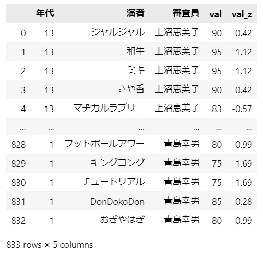
There are 833 rows in total.
The items are: "Year": tournament edition, "Performer": comedy duo name, "Judge": judge name, "val": evaluation score, "val_z": standardized evaluation score.
3. Data Overview and Statistics
First, let's check the summary statistics.
### 要約統計量の表示
data.describe().round(3)
[Execution Result]
The evaluation scores (val) seem to take a wide range of values from 50 to 100.

4. Drawing Box Plots
We will create box plots using seaborn's boxplot.
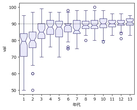
The first one is the evaluation score by tournament edition.
### 箱ひげ図のプロット1 開催回別評価得点
plt.figure(figsize=(5, 4))
sns.boxplot(data=data, x='年代', y='val', notch=True, linewidth=0.8,
            color='lavender', linecolor='midnightblue')
plt.axhline(90, color='black', lw=0.5, ls='--');
[Execution Result]
It seems there was significant variation in the first few editions immediately after the start.
Next, the evaluation scores by comedy duo.
### 箱ひげ図のプロット2 コンビ別評価得点
plt.figure(figsize=(15, 4))
sns.boxplot(data=data, x='演者', y='val', notch=True, linewidth=0.8,
            color='lavender', linecolor='midnightblue')
plt.axhline(90, color='black', lw=0.5, ls='--')
plt.xticks(rotation=270);
[Execution Result]
Some names have been omitted.
Scores below 90 do not seem to be rare.

Finally, the evaluation scores by judge.
### 箱ひげ図のプロット3 審査員別評価得点
plt.figure(figsize=(8, 4))
sns.boxplot(data=data, x='審査員', y='val', notch=True, linewidth=0.8,
            color='lavender', linecolor='midnightblue')
plt.axhline(90, color='black', lw=0.5, ls='--')
plt.xticks(rotation=270);
[Execution Result]
Some names have been omitted.
It can be seen that there are differences in variation depending on the judge.

5. Data Preprocessing
We will obtain the elements and indices of the categorical variables.
These data are used within the PyMC model.
### カテゴリ変数の要素とインデックスの取得
combi_cat = pd.Categorical(data['演者']).categories
combi_idx = pd.Categorical(data['演者']).codes
judge_cat = pd.Categorical(data['審査員']).categories
judge_idx = pd.Categorical(data['審査員']).codes
times_cat = pd.Categorical(data['年代']).categories
times_idx = pd.Categorical(data['年代']).codes
Model 1: Duo Average Model
This is the model from the text "11.2 Duo Average Model".
Mathematical Representation of the Model
This is a "pseudo-mathematical" notation that mixes the atmosphere of the PyMC model we aim for.
The subscript $${i}$$ is the index of the duo.
Also, since the prior distributions for $${θ_i}$$ and $${σ_i}$$ are not explicitly stated in the text, we set sufficiently wide parameters.
$$
\begin{align*}
\theta_i &\sim \text{Uniform}\ (\text{lower}=-100,\ \text{upper}=100) \\
\sigma_i &\sim \text{HalfCauchy}\ (\text{beta}=100) \\
likelihood &\sim \text{Normal}\ (\text{mu}=\theta_i,\ \text{sigma}=\sigma_i) \\
\end{align*}
$$
1. Definition of the Model
### モデルの定義

with pm.Model() as model1:

    ### データ関連定義
    # coordの定義
    model1.add_coord('data', values=data.index, mutable=True)
    model1.add_coord('combi', values=combi_cat, mutable=True)
    # dataの定義
    y = pm.ConstantData('y', value=data['val_z'].values, dims='data')

    ### 事前分布
    # 事前分布
    theta = pm.Uniform('theta', lower=-100, upper=100, dims='combi')
    sigma = pm.Uniform('sigma', lower=0, upper=100, dims='combi')

    ### 尤度
    likelihood = pm.Normal('likelihood',
                           mu=theta[combi_idx], sigma=sigma[combi_idx],
                           observed=y, dims='data')
[Model Annotation] Omitted
2. Checking the Model Overview
### モデルの表示
model1
[Execution Result]
It is a simple model.

# モデルの可視化
pm.model_to_graphviz(model1)
[Execution Result]
It is a simple model.

3. Sampling from the Posterior Distribution
The number of random number generations (draws) is fewer than in the text.
By setting nuts_sampler='numpyro', you can use numpyro as the NUTS sampler.
The processing time was approximately 30 seconds.
### 事後分布からのサンプリング ※NUTSサンプラーにnumpyroを使用 30秒
with model1:
    idata1 = pm.sample(draws=5000, tune=5000, chains=4, target_accept=0.9,
                       nuts_sampler='numpyro', random_seed=123)
[Execution Result] Omitted
4. Checking Sampling Data
Check $$\hat{R}$$ and trace plots.
Convergence of the posterior distribution is confirmed with $$\hat{R}\leq 1.1$$.
### r_hat>1.1の確認
rhat_idata1 = az.rhat(idata1)
(rhat_idata1>1.1).sum()
[Execution Result]
There are "0" parameters with $$\hat{R} >1.1$$.
We have confirmed that all parameters satisfy $$\hat{R} \leq 1.1$$.

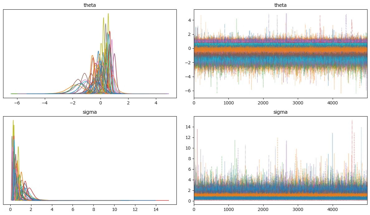
These are the trace plots.
### トレースプロットの表示
pm.plot_trace(idata1, compact=True, combined=True, figsize=(12, 7))
plt.tight_layout();
[Execution Result]
The dense appearance makes it look as if the parameters are competing with each other.
5. Results of the Duo Average Model
Calculate the "summary statistics of the top 5 pairs for the posterior distribution of funniness ($$\theta_i$$)" corresponding to Table 11.1 in the text.
We will use the pm.summary() function for this.
### おもしろさの事後分布の上位5組の要約統計情報 ★表11.1に対応
(pm.summary(idata1, hdi_prob=0.95, kind='stats', var_names=['theta'])
 .sort_values('mean', ascending=False).head(5).reset_index().round(2))
[Execution Result]
The order matches the text.
The mean (EAP in the text) differs slightly from the text.
The standard deviation (sd, post.sd in the text) differs from the text.
Note that the lower and upper bounds differ because the text uses credible intervals, while this article uses HDI.

Next, we calculate the "median and 95% credible interval of the posterior distribution of standard deviation" corresponding to Table 11.2 in the text.
### 標準偏差の事後分布の中央値および95%信用区間 ★表11.2に対応

# 推論データから要約統計情報を計算する関数の定義
def calc_stat(i, idata):
    tmp = idata.posterior.sigma[:, :, i].data.flatten()
    return [combi_cat[i], np.median(tmp), np.quantile(tmp, 0.025),
            np.quantile(tmp, 0.975)]

## sigma_statsデータフレームの作成
# データフレームの初期化
sigma_stats = pd.DataFrame()
# top5の順に要約統計情報を計算してデータフレームに追加
for i in set(combi_idx):
    tmp_stats = calc_stat(i, idata1)
    sigma_stats = pd.concat([sigma_stats, pd.DataFrame(tmp_stats).T], axis=0)
# カラム名とインデックスの補正(型をfloatに変換の上、中央値で降順ソート)
sigma_stats.columns = ['コンビ名', '中央値', '2.5%', '97.5%']
sigma_stats = sigma_stats.astype({'中央値': float, '2.5%': float, '97.5%': float})
sigma_stats = sigma_stats.sort_values(by='中央値', ascending=False)
sigma_stats.reset_index(drop=True, inplace=True)

# 要約統計量の表示
print('【標準偏差の事後分布の中央値と95%信用区間】')
display(sigma_stats.head(3).round(2))
display(sigma_stats.tail(3).round(2))
[Execution Result]
The order matches the text.
The median and credible interval values differ slightly from the text.
In the box-and-whisker plot for each duo shown earlier, the duos with larger interval widths (i.e., greater variance in scores) are ranked higher.

6. Saving Inference Data (idata)
Let's save the inference data to a file in case we need to reuse it.
We will save idata1 using pickle.
### idataの保存 pickle
file = r'idata1_ch11.pkl'
with open(file, 'wb') as f:
    pickle.dump(idata1, f)
The code for loading is as follows.
### idataの読み込み pickle
file = r'idata1_ch11.pkl'
with open(file, 'rb') as f:
    idata1_load = pickle.load(f)
Model 2: Judge Bias Evaluation Model
This is the model from "11.3 Judge Bias Evaluation Model" in the text.
Mathematical Representation of the Model
This is a "pseudo-mathematical" notation that incorporates the feel of the PyMC model we want to achieve.
The subscript $$i$$ is the index for the duo, and $$j$$ is the index for the judge.
$$
\begin{align*}
\sigma_{\theta_i} &\sim \text{HalfCaushy}\ (\text{beta}=5)\\
\theta_i &\sim \text{Normal}\ (\text{mu}=0,\ \text{sigma}=\sigma_{\theta_i}) \\
\sigma_j &\sim \text{HalfCauchy}\ (\text{beta}=5) \\
likelihood &\sim \text{Normal}\ (\text{mu}=\theta_i,\ \text{sigma}=\sigma_j) \\
\end{align*}
$$
1. Model Definition
### モデルの定義

with pm.Model() as model2:

    ### データ関連定義
    # coordの定義
    model2.add_coord('data', values=data.index, mutable=True)
    model2.add_coord('combi', values=combi_cat, mutable=True)
    model2.add_coord('judge', values=judge_cat, mutable=True)
    # dataの定義
    y = pm.ConstantData('y', value=data['val_z'].values, dims='data')

    ### 事前分布
    # 事前分布
    sigmaTheta = pm.HalfCauchy('sigmaTheta', beta=5, dims='combi')
    theta = pm.Normal('theta', mu=0, sigma=sigmaTheta, dims='combi')
    sigma = pm.HalfCauchy('sigma', beta=5, dims='judge')

    ### 尤度
    likelohood = pm.Normal('likelihood',
                           mu=theta[combi_idx], sigma=sigma[judge_idx],
                           observed=y, dims='data')
[Model Annotation] Omitted
2. Checking the Model Structure
### モデルの表示
model2
[Execution Result]
This is a simple model.

# モデルの可視化
pm.model_to_graphviz(model2)
[Execution Result]
This is a simple model.

3. Sampling from the Posterior Distribution
The number of draws is lower than in the text.
By setting nuts_sampler='numpyro', you can use numpyro as the NUTS sampler.
The processing time was approximately 50 seconds.
### 事後分布からのサンプリング ※NUTSサンプラーにnumpyroを使用 50秒
with model2:
    idata2 = pm.sample(draws=5000, tune=5000, chains=4, target_accept=0.9,
                       nuts_sampler='numpyro', random_seed=1235)
[Execution Result] Omitted
4. Checking Sampling Data
Check the $$\hat{R}$$ and trace plots.
The convergence of the posterior distribution is confirmed with $$\hat{R}\leq 1.1$$.
### r_hat>1.1の確認
rhat_idata2 = az.rhat(idata2)
(rhat_idata2>1.1).sum()
[Execution Result]
There are 0 parameters with $$\hat{R} >1.1$$.
I was able to confirm that all parameters satisfy $$\hat{R} \leq 1.1$$.

These are the trace plots.
### トレースプロットの表示
pm.plot_trace(idata2, compact=True, combined=True, figsize=(12, 7))
plt.tight_layout();
[Execution Result]
The dense appearance makes it look as if the parameters are competing with each other.
I am concerned about the many black lines at the bottom (commonly known as barcodes) indicating divergence.

5. Results of the Judge Bias Evaluation Model
Calculate the 'Summary statistics of the top 5 pairs for funniness ($$\theta_i$$) posterior distribution', which corresponds to Table 11.3 in the text.
This is handled by the pm.summary() function.
### おもしろさの事後分布の上位5組の要約統計情報 ★表11.3に対応
(pm.summary(idata2, hdi_prob=0.95, kind='stats', var_names=['theta'])
 .sort_values('mean', ascending=False).head(5).reset_index().round(2))
[Execution Result]
There is a slight difference from the order in the text.
The slight discrepancy with the text regarding the mean (EAP in the text) seems to have affected the order.
The standard deviation (sd, post.sd in the text) also differs slightly from the text.
Note that for the lower and upper bounds, the results differ because the text uses credible intervals, while this article uses HDI.

Next, calculate the 'Median and 95% credible interval of the posterior distribution of standard deviation', which corresponds to Table 11.4 in the text.
### 標準偏差の事後分布の中央値および95%信用区間 ★表11.4に対応

## 推論データから要約統計情報を計算する関数の定義
def calc_stat(i, idata):
    tmp = idata.posterior.sigma[:, :, i].data.flatten()
    return [judge_cat[i], np.median(tmp), np.quantile(tmp, 0.025),
            np.quantile(tmp, 0.975)]

## sigma_statsデータフレームの作成
# データフレームの初期化
sigma_stats = pd.DataFrame()
# top5の順に要約統計情報を計算してデータフレームに追加
for i in set(judge_idx):
    tmp_stats = calc_stat(i, idata2)
    sigma_stats = pd.concat([sigma_stats, pd.DataFrame(tmp_stats).T], axis=0)
# カラム名とインデックスの補正(型をfloatに変換の上、中央値で降順ソート)
sigma_stats.columns = ['審査員', '中央値', '2.5%', '97.5%']
sigma_stats = sigma_stats.astype({'中央値': float, '2.5%': float, '97.5%': float})
sigma_stats = sigma_stats.sort_values(by='中央値', ascending=False)
sigma_stats.reset_index(drop=True, inplace=True)

# 要約統計量の表示
print('【標準偏差の事後分布の中央値と95%信用区間】')
display(sigma_stats.head(3).round(2))
display(sigma_stats.tail(3).round(2))
[Execution Result]
The order matches the text.
The values for the median and credible intervals differ slightly from the text.
In the box-and-whisker plots for each judge shown earlier, the judges with wider intervals (i.e., greater variance in scores) are ranked higher.

6. Saving Inference Data (idata)
Let's save the inference data to a file in case we need to reuse it.
Save idata2 using pickle.
### idataの保存 pickle
file = r'idata2_ch11.pkl'
with open(file, 'wb') as f:
    pickle.dump(idata2, f)
The code for loading is as follows.
### idataの読み込み pickle
file = r'idata2_ch11.pkl'
with open(file, 'rb') as f:
    idata2_load = pickle.load(f)
Model 3: Judge Criterion Effect Model
This is the model from '11.4 Judge Criterion Effect Model' in the text.
Mathematical Representation of the Model
This is a 'pseudo-mathematical' notation that mixes in the feel of the PyMC model I want to achieve.
The subscript $${i}$$ is the index for the pair, and $${j}$$ is the index for the judge.
$$
\begin{align*}
\sigma_{\theta} &\sim \text{HalfCaushy}\ (\text{beta}=5)\\
\sigma_{\gamma} &\sim \text{HalfCaushy}\ (\text{beta}=5)\\
\sigma_i &\sim \text{HalfCauchy}\ (\text{beta}=5) \\
\theta_i &\sim \text{Normal}\ (\text{mu}=0,\ \text{sigma}=\sigma_{\theta}) \\
\gamma_j &\sim \text{Normal}\ (\text{mu}=0,\ \text{sigma}=\sigma_{\gamma}) \\
likelihood &\sim \text{Normal}\ (\text{mu}=\theta_i + \gamma_j,\ \text{sigma}=\sigma_i) \\
\end{align*}
$$
1. Model Definition
### モデルの定義

with pm.Model() as model3:

    ### データ関連定義
    # coordの定義
    model3.add_coord('data', values=data.index, mutable=True)
    model3.add_coord('combi', values=combi_cat, mutable=True)
    model3.add_coord('judge', values=judge_cat, mutable=True)
    # dataの定義
    y = pm.ConstantData('y', value=data['val_z'].values, dims='data')

    ### 事前分布
    # θ_i, σ_θ
    sigmaTheta = pm.HalfCauchy('sigmaTheta', beta=5)
    theta = pm.Normal('theta', mu=0, sigma=sigmaTheta, dims='combi')
    # γ_j, σ_γ
    sigmaGamma = pm.HalfCauchy('sigmaGamma', beta=5)
    gamma = pm.Normal('gamma', mu=0, sigma=sigmaGamma, dims='judge')
    # σ_i
    sigma = pm.HalfCauchy('sigma', beta=5, dims='combi')

    ### 尤度
    likelohood = pm.Normal('likelihood',
                           mu=theta[combi_idx] + gamma[judge_idx],
                           sigma=sigma[combi_idx], observed=y, dims='data')
[Model Annotation] Omitted
2. Checking the Model Appearance
### モデルの表示
model3
[Execution Result]
It is still a simple model.

# モデルの可視化
pm.model_to_graphviz(model2)
[Execution Result]
It is still a simple model.

3. Sampling from the Posterior Distribution
The number of draws is smaller than in the text.
By setting nuts_sampler='numpyro', you can use numpyro as the NUTS sampler.
The processing time was approximately 20 seconds.
### 事後分布からのサンプリング ※NUTSサンプラーにnumpyroを使用 20秒
with model3:
    idata3 = pm.sample(draws=5000, tune=5000, chains=4, target_accept=0.9,
                       nuts_sampler='numpyro', random_seed=1235)
[Execution Result] Omitted
4. Checking Sampling Data
Check the $$\hat{R}$$ and trace plots.
The convergence check for the posterior distribution is set to $$\hat{R}\leq 1.1$$.
### r_hat>1.1の確認
rhat_idata3 = az.rhat(idata3)
(rhat_idata3>1.1).sum()
[Execution Result]
There are "0" parameters with $$\hat{R} >1.1$$.
I have confirmed that all parameters satisfy $$\hat{R} \leq 1.1$$.

This is the trace plot.
### トレースプロットの表示
pm.plot_trace(idata3, compact=True, combined=True, figsize=(12, 7))
plt.tight_layout();
[Execution Result]
The way they are clustered makes it look as if the parameters are competing with each other.

5. Results of the Judge Criterion Effect Model
Calculate the "summary statistics of the top 5 pairs for funniness ($$\theta_i$$)" corresponding to Table 11.5 in the text.
This is handled by the pm.summary() function.
### おもしろさの事後分布の上位5組の要約統計情報 ★表11.5に対応
(pm.summary(idata3, hdi_prob=0.95, kind='stats', var_names=['theta'])
 .sort_values('mean', ascending=False).head(5).reset_index().round(2))
[Execution Result]
The order seems quite different from the text.
It appears that the mean (EAP in the text) is lower than in the text.
The reason is unknown...
Note that regarding the lower and upper bounds, the results differ because the text uses credible intervals, while this article uses HDI.

Next, calculate the "summary statistics of the posterior distribution of evaluation criteria" corresponding to Table 11.6 in the text.
### 評価基準の事後分布の要約統計情報 ★表11.6に対応

## 推論データから要約統計情報を計算する関数の定義
def calc_stat(i, idata):
    tmp = idata.posterior.gamma[:, :, i].data.flatten()
    return [judge_cat[i], np.mean(tmp), np.std(tmp), np.quantile(tmp, 0.025),
            np.quantile(tmp, 0.975)]

## gamma_statsデータフレームの作成
# データフレームの初期化
gamma_stats = pd.DataFrame()
# top5の順に要約統計情報を計算してデータフレームに追加
for i in set(judge_idx):
    tmp_stats = calc_stat(i, idata3)
    gamma_stats = pd.concat([gamma_stats, pd.DataFrame(tmp_stats).T], axis=0)
# カラム名とインデックスの補正(型をfloatに変換の上、EAPで降順ソート)
gamma_stats.columns = ['審査員', 'EAP', 'post.sd', '2.5%', '97.5%']
gamma_stats = gamma_stats.astype({'EAP': float, 'post.sd': float,
                                  '2.5%': float, '97.5%': float})
gamma_stats = gamma_stats.sort_values(by='EAP', ascending=False)
gamma_stats.reset_index(drop=True, inplace=True)

## 要約統計量の表示
print('【評価基準の事後分布の要約統計量】')
display(gamma_stats.head(3).round(2))
display(gamma_stats.tail(3).round(2))
[Execution Result]
This matches the order in the text.
The median and credible interval values are almost identical to the text.

6. Saving Inference Data (idata)
Let's save the inference data to a file in case we need to reuse it.
Save idata3 using pickle.
### idataの保存 pickle
file = r'idata3_ch11.pkl'
with open(file, 'wb') as f:
    pickle.dump(idata3, f)
The code for loading is as follows.
### idataの読み込み pickle
file = r'idata3_ch11.pkl'
with open(file, 'rb') as f:
    idata3_load = pickle.load(f)
Model 4: Tournament Count Effect Model
This is the model from "11.5 Tournament Count Effect Model" in the text.
Mathematical Representation of the Model
This is a "pseudo-mathematical" notation that incorporates the feel of the PyMC model I want to aim for.
The subscript $$i$$ is the index for the duo, $$j$$ is the index for the judge, and $$o$$ is the index for the tournament count.
$$
\begin{align*}
\sigma_{\theta} &\sim \text{HalfCaushy}\ (\text{beta}=5)\\
\sigma_{\gamma} &\sim \text{HalfCaushy}\ (\text{beta}=5)\\
\sigma_{\zeta} &\sim \text{HalfCaushy}\ (\text{beta}=5)\\
\sigma_e &\sim \text{HalfCauchy}\ (\text{beta}=5) \\
\theta_i &\sim \text{Normal}\ (\text{mu}=0,\ \text{sigma}=\sigma_{\theta}) \\
\gamma_j &\sim \text{Normal}\ (\text{mu}=0,\ \text{sigma}=\sigma_{\gamma}) \\
\zeta_o &\sim \text{Normal}\ (\text{mu}=0,\ \text{sigma}=\sigma_{\zeta}) \\
likelihood &\sim \text{Normal}\ (\text{mu}=\theta_i + \gamma_j + \zeta_o,\ \text{sigma}=\sigma_e) \\
\end{align*}
$$
1. Model Definition
### モデルの定義

with pm.Model() as model4:

    ### データ関連定義
    # coordの定義
    model4.add_coord('data', values=data.index, mutable=True)
    model4.add_coord('combi', values=combi_cat, mutable=True)
    model4.add_coord('judge', values=judge_cat, mutable=True)
    model4.add_coord('times', values=times_cat, mutable=True)
    # dataの定義
    y = pm.MutableData('y', value=data['val_z'].values, dims='data')

    ### 事前分布
    # θ_i, σ_θ
    sigmaTheta = pm.HalfCauchy('sigmaTheta', beta=5)
    theta = pm.Normal('theta', mu=0, sigma=sigmaTheta, dims='combi')
    # γ_j, σ_γ
    sigmaGamma = pm.HalfCauchy('sigmaGamma', beta=5)
    gamma = pm.Normal('gamma', mu=0, sigma=sigmaGamma, dims='judge')
    # ζ_j, σ_ζ
    sigmaZeta = pm.HalfCauchy('sigmaZeta', beta=5)
    zeta = pm.Normal('zeta', mu=0, sigma=sigmaZeta, dims='times')
    # σ_e
    sigmaE = pm.HalfCauchy('sigmaE', beta=5)

    ### 尤度
    likelohood = pm.Normal('likelihood',
                    mu=theta[combi_idx] + gamma[judge_idx] + zeta[times_idx],
                    sigma=sigmaE, observed=y, dims='data')
[Model Annotation] Omitted
2. Checking the Model Appearance
### モデルの表示
model4
[Execution Result]
The number of prior distributions has increased.

# モデルの可視化
pm.model_to_graphviz(model4)
[Execution Result]
You can clearly see how parameters are set for each duo (combi), judge, and tournament year (times).

3. Sampling from the Posterior Distribution
The number of draws is lower than in the text.
By setting nuts_sampler='numpyro', you can use numpyro as the NUTS sampler.
The processing time was approximately 20 seconds.
### 事後分布からのサンプリング ※NUTSサンプラーにnumpyroを使用 20秒
with model4:
    idata4 = pm.sample(draws=5000, tune=5000, chains=4, target_accept=0.9,
                       nuts_sampler='numpyro', random_seed=1235)
[Execution Result] Omitted
4. Checking Sampling Data
Check the R-hat and trace plots.
Convergence of the posterior distribution is checked with R-hat <= 1.1.
### r_hat>1.1の確認
rhat_idata4 = az.rhat(idata4)
(rhat_idata4>1.1).sum()
[Execution Result]
There are 0 parameters with R-hat > 1.1.
We have confirmed that all parameters have R-hat <= 1.1.

These are the trace plots.
### トレースプロットの表示
pm.plot_trace(idata4, compact=True, combined=True, figsize=(12, 10))
plt.tight_layout();
[Execution Result]
The clean figures clearly show that the model has converged.

5. Results of the Tournament Year Effect Model
Calculate the 'summary statistics of the posterior distribution of funniness (theta_i)', which corresponds to Table 11.7 in the text.
### おもしろさの事後分布の要約統計情報 ★表11.7に対応

## 推論データから要約統計情報を計算する関数の定義
def calc_stat(i, idata):
    tmp = idata.posterior.theta[:, :, i].data.flatten()
    return [combi_cat[i], np.mean(tmp), np.std(tmp), np.quantile(tmp, 0.025),
            np.quantile(tmp, 0.975)]

## theta_statsデータフレームの作成
# データフレームの初期化
theta_stats = pd.DataFrame()
# top5の順に要約統計情報を計算してデータフレームに追加
for i in set(combi_idx):
    tmp_stats = calc_stat(i, idata4)
    theta_stats = pd.concat([theta_stats, pd.DataFrame(tmp_stats).T], axis=0)
# カラム名とインデックスの補正(型をfloatに変換の上、EAPで降順ソート)
theta_stats.columns = ['コンビ名', 'EAP', 'post.sd', '2.5%', '97.5%']
theta_stats = theta_stats.astype({'EAP': float, 'post.sd': float,
                                  '2.5%': float, '97.5%': float})
theta_stats = theta_stats.sort_values(by='EAP', ascending=False)
theta_stats.reset_index(drop=True, inplace=True)
theta_stats.index = theta_stats.index + 1

## 要約統計量の表示
print('【おもしろさ(θ)の事後分布の要約統計量】')
display(theta_stats.head(31).round(2))
display(theta_stats.tail(31).round(2))
[Execution Result]
It seems that the early winning duos are at the top.
Note that there are some differences from the order in the text.
The text performs sorting after rounding to two decimal places, whereas this code performs rounding after sorting.
This difference in processing likely has an impact.
Please refer to the text for the substantive analysis!

Next, we calculate the 'summary statistics of the posterior distribution of judges' evaluation criteria (gamma_j)', which corresponds to Table 11.8 in the text.
### 審査員の審査基準の事後分布の要約統計情報 ★表11.8に対応

## 推論データから要約統計情報を計算する関数の定義
def calc_stat(i, idata):
    tmp = idata.posterior.gamma[:, :, i].data.flatten()
    return [judge_cat[i], np.mean(tmp), np.std(tmp), np.quantile(tmp, 0.025),
            np.quantile(tmp, 0.975)]

## gamma_statsデータフレームの作成
# データフレームの初期化
gamma_stats = pd.DataFrame()
# top5の順に要約統計情報を計算してデータフレームに追加
for i in set(judge_idx):
    tmp_stats = calc_stat(i, idata4)
    gamma_stats = pd.concat([gamma_stats, pd.DataFrame(tmp_stats).T], axis=0)
# カラム名とインデックスの補正(型をfloatに変換の上、EAPで降順ソート)
gamma_stats.columns = ['審査員', 'EAP', 'post.sd', '2.5%', '97.5%']
gamma_stats = gamma_stats.astype({'EAP': float, 'post.sd': float,
                                  '2.5%': float, '97.5%': float})
gamma_stats = gamma_stats.sort_values(by='EAP', ascending=False)
gamma_stats.reset_index(drop=True, inplace=True)
gamma_stats.index = gamma_stats.index + 1

## 要約統計量の表示
print('【審査員の審査基準(γ)の事後分布の要約統計量】')
display(gamma_stats.head(13).round(2))
display(gamma_stats.tail(14).round(2))
[Execution Result]
There are some differences from the order in the text.
Here too, the timing of the sorting process is thought to be affecting the difference in order.
Please refer to the text for the substantive analysis!

6. Effect of Tournament Year
Plot the 'tournament year (zeta_o) and posterior distribution interval estimation', which corresponds to Figure 11.1 in the text.
A forest plot was used.
### フォレストプロットの描画 ★図11.1に対応
ax = pm.plot_forest(idata4, var_names=['zeta'], hdi_prob=0.95, combined=True,
                    figsize=(6,4))
ax[0].set_title(r'開催回数($\zeta_o$)の事後分布の区間推定結果')
ax[0].set_xlabel('EAP推定値', fontsize=14)
ax[0].set_ylabel('開催回数', fontsize=14);
[Execution Result]
In the early years of the tournament, the values were negative, showing an effect of lowering the average evaluation score.

7. Plotting the Reliability of Funniness
Plot the 'posterior distribution of the reliability of funniness (rho_theta)', which corresponds to Figure 11.2 in the text.
We use seaborn's histplot.
### おもしろさの信頼性の事後分布 ★図11.2に対応

# ρ_θの計算
sigma_theta_data = idata4.posterior.sigmaTheta.data.flatten()
sigma_gamma_data = idata4.posterior.sigmaGamma.data.flatten()
sigma_e_data = idata4.posterior.sigmaE.data.flatten()
rho = (sigma_theta_data**2
       / (sigma_theta_data**2 + sigma_gamma_data**2 + sigma_e_data**2))

# 95%区間の計算
q025 = np.quantile(rho, 0.025)
q975 = np.quantile(rho, 0.975)

# ρのヒストグラムの描画
ax = sns.histplot(rho, bins=100, stat='density', kde=True)
# 95%境界線の描画
ax.axvline(q025, lw=1, ls='--', color='black', label='95%境界線')
ax.axvline(q975, lw=1, ls='--', color='black')
# 修飾
ax.set_title(r'おもしろさの信頼性($\rho_{\theta}$)の事後分布')
ax.set_xlabel(r'$\rho_{\theta}$')
ax.set_ylabel('確率密度')
ax.legend();
[Execution Result]
Borrowing from the analysis in the text, assuming this model is the true model, the argument is that 'at most about 30% is determined by the funniness of the manzai'.
The upper bound of the 95% confidence interval is approximately 0.34.

8. Saving Inference Data (idata)
Let's save the inference data to a file in case we need to reuse it.
Save idata4 using pickle.
### idataの保存 pickle
file = r'idata4_ch11.pkl'
with open(file, 'wb') as f:
    pickle.dump(idata4, f)
The code for loading is as follows.
### idataの読み込み pickle
file = r'idata4_ch11.pkl'
with open(file, 'rb') as f:
    idata4_load = pickle.load(f)
This concludes Chapter 11.
Conclusion
A simple model
It was a very educational modeling experience where I could feel the persuasiveness that comes precisely because it is a simple model.
Models where the normal distribution exerts its power feel incredibly invincible!
If only the world were generated by a bell curve + white noise...

Series articles
Next article
Previous article
Table of contents
Blog introduction
I am writing four series of articles on note.
Please come and take a look!
1. Relaxed Statistics
This is a blog that roughly explores probability and statistics using the Statistics Certification Grade 2 problem collection as a guide.
Feel free to read it as if it were casual conversation. Please come and take a look.
It corresponds to the Statistics Certification Grade 2 Official Problem Collection CBT version.
2. Introduction to Time Series Analysis for Psychology starting with R and Stan, using Python and PyMC Ver. 5
I am tackling the time series analysis topics from the book 'Introduction to Time Series Analysis for Psychology starting with R and Stan' using Python and PyMC Ver. 5.
I believe that practicing with a wealth of themes (topics) will lead to building basic strength in Python and PyMC.
Every day, I work hard at web searching, understanding time series models, grasping Python packages, and translating R/Stan code!
I hope this series will be a reference for beginners in Python time series analysis 🍀
3. Python Machine Learning Programming Practice Log
I wrote articles about my various thoughts when I studied the book 'Python Machine Learning Programming: PyTorch & scikit-learn Edition'.
This book is a textbook for scikit-learn and PyTorch.
Please feel free to try it out if you like.
4. Writing about things that seem like data science
I write columns on statistics, data analysis, AI, machine learning, and Python on an irregular basis.
Series on 'Statistics', 'Python', 'Mathematics and Python', and 'R' have been created.
Practical records of Bayesian books are also posted.
Thank you very much for reading until the end.
いいなと思ったら応援しよう!
 応援ありがとうございます。これからもがんばって記事を作成します!