10-2-4 Analysis of Variance for Multiple Regression Models - The final problem of the CBT-compatible version (Final Episode)

This statistical topic

This is the final problem on analysis of variance.
In fact, analysis of variance is the final theme of the CBT-compatible problem collection.
Therefore, this article is the final episode.
Let's enjoy the connection between multiple regression models and one-way ANOVA tables.

Preparation of the official problem collection

We will use the problems from the "Official Problem Collection". Please have the official problem collection at hand.
If you do not have the official problem collection, do not worry!
Please enjoy statistics at your leisure in the "Learn" and "Practice" chapters!

Structure of this article

This article will have a different chapter structure than the usual articles.
We will combine "Solving Problems" and "Learning" into one chapter.
In the following "Practice" section, we will perform multiple regression analysis and analysis of variance using rent data in Python, EXCEL, and R.

Learning while solving problems

📘 Official Problem Collection Category

Field of Linear Models - Field of Analysis of Variance
Question 4 Analysis of Variance for Multiple Regression Models (Rent of Rental Apartments)

Exam Date
Under investigation

📕 Official Textbook
・5.1.7 Test of Significance of Regression and Test of Regression Coefficients (from page 175)
・5.2.1 One-way Analysis of Variance (from page 185)

Problem

Please refer to the official problem collection.

How to solve

Intent of the question
Regarding the multiple regression model, we will answer the following two questions based on the "statistical software output results" and the "one-way ANOVA table (with blanks)" described in the problem statement.
Question 1. Filling in the blanks of the one-way ANOVA table
Question 2. Test of significance of regression

Question 1: Filling in the blanks of the one-way ANOVA table

Although it has already been calculated in the problem statement, we will re-confirm the connection between the statistical software output results and the one-way ANOVA table.

Given the standard error of the residuals of $${9.904}$$, the degrees of freedom of $${185}$$, and the formula for the standard error of the residuals, we can find the sum of squares of the residuals.
Given the coefficient of determination of $${0.8512}$$, the sum of squares of the residuals, and the formula for the coefficient of determination, we can find the total sum of squares.
Through the sum of squares and degrees of freedom, the output results of statistical software are linked to the one-way ANOVA table!

Now, let's proceed to fill in the blanks of the one-way ANOVA table!
The calculation mechanism for the one-way ANOVA table of a regression model is as follows.

$$
\begin{array}{|c|c:c:c:c|}
\hline
Source of Variation & Sum of Squares & Degrees of Freedom & Mean Square & F \\
\hline
Regression & S_R & p & V_R = S_R / p & F = V_R / V_e \\
\hdashline
Residual & S_e & n-p-1 & V_e = S_e / (n-p-1) & - \\
\hline
Total & S_T & n-1 & - & - \\
\hline
\end{array}
$$

The degrees of freedom for the sum of squares due to regression is the number of explanatory variables, $${p}$$.
The multiple regression model has two explanatory variables: "room size" and "age of the building."
Therefore, the degrees of freedom for the sum of squares due to regression is $${2}$$.

Let's enter what we have found so far into the one-way ANOVA table.

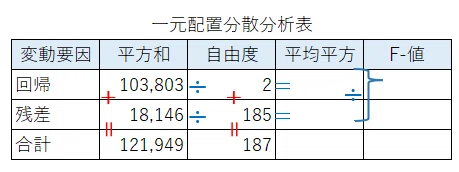
The "Mean Square" and "F-value" are calculated by performing the division shown in blue.

We have completed all the calculations.
Let's complete the one-way ANOVA table.

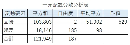
For the answer choices, (a) the degrees of freedom for regression is $${2}$$, and (e) the F-value is $${529}$$.

The answer to Question 1 is ③.

Question 2. Test for significance of regression

Using the one-way ANOVA table, we will perform a test for the significance of the regression at a significance level of $${5\%}$$.

The $${F}$$-value in the one-way ANOVA table follows an $${F}$$-distribution with degrees of freedom $${(p, n-p-1)}$$.

Let's confirm the formula for the ANOVA table of a multiple regression model.

$$
\begin{array}{|c|c:c:c:c|}
\hline
Source of Variation & Sum of Squares & Degrees of Freedom & Mean Square & F \\
\hline
Regression & S_R & p & V_R = S_R / p & F = V_R / V_e \\
\hdashline
Residual & S_e & n-p-1 & V_e = S_e / (n-p-1) & - \\
\hline
Total & S_T & n-1 & - & - \\
\hline
\end{array}
$$

The numerator of the $${F}$$-value is the mean square of the regression, and the denominator is the mean square of the residuals.
Regarding the degrees of freedom, $${p}$$ on the numerator side is the first degree of freedom, and $${n-p-1}$$ on the denominator side is the second degree of freedom.

Let's also confirm the formula for the $${F}$$-test statistic.

$$
F=\cfrac{V_R}{V_e}=\cfrac{S_R/p}{S_e/(n-p-1)}=\cfrac{(S_R/\sigma^2)/p}{(S_e/\sigma^2)/(n-p-1)} \sim F(p, n-p-1)
$$

The $${F}$$-test statistic follows an $${F}$$-distribution with degrees of freedom $${(p, n-p-1)}$$.
The first degree of freedom is $${p}$$, and the second degree of freedom is $${n-p-1}$$.

Applying this to the current problem, the degrees of freedom for regression, which is the first degree of freedom, is $${2}$$, and the degrees of freedom for residuals, which is the second degree of freedom, is $${185}$$.

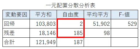
Among the answer choices, only (3) includes the degrees of freedom $${(2, 185)}$$.

The answer to Question 2 is (3).

Continuation of 'Test for Significance of Regression'

Let's continue with the test for the significance of regression.

From the percentage point table of the $${F}$$ distribution, let's obtain the upper $${5\%}$$ point for degrees of freedom $${(2, 185)}$$.

The maximum value for the second degree of freedom is $${120}$$.
Looking at other columns, as the value of the second degree of freedom increases, the value of the upper $${5\%}$$ point decreases.
In other words, the upper $${5\%}$$ point for a second degree of freedom of $${185}$$ is smaller than the upper $${5\%}$$ point for $${120}$$.
If the upper $${5\%}$$ point is larger, the rejection region becomes smaller, and the null hypothesis becomes harder to reject.
The hurdle for the test becomes higher.

Here, let's use $${3.072}$$, which is the upper $${5\%}$$ point for the second degree of freedom of $${120}$$, where the hurdle is higher.

The $${F}$$ value is $${529}$$, which is larger than the upper $${5\%}$$ point of $${3.072}$$.
In other words, the null hypothesis is rejected at the $${5\%}$$ significance level.

[Conclusion]
The null hypothesis is rejected at the $${5\%}$$ significance level, and we can say that the alternative hypothesis 'the regression is significant' holds.

'The regression is significant' means that 'at least one of the regression coefficients in the regression model is not zero' or 'there is an explanatory variable that affects the objective variable'.

Let's plot the $${F}$$ value and the upper $${5\%}$$ point on the graph of the $${F}$$ distribution with degrees of freedom $${(2, 185)}$$ to confirm that the $${F}$$ value is included in the rejection region.

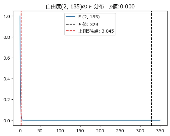
The $${F}$$ value, indicated by the black dotted line, is included in the rejection region above the upper $${5\%}$$ point, indicated by the red dotted line!
The $${p}$$ value is 0.000, and the upper $${5\%}$$ point is $${3.045}$$.

Finalizing the One-Way ANOVA Table

Let's finalize the one-way ANOVA table.

'Test for Significance of Regression Coefficients'

Changing our perspective slightly, let's consider the 'test for significance of regression coefficients'.

The values of the regression coefficients for the multiple regression model are as follows.

Testing whether each of these regression coefficients is "not zero = affects the objective variable" is the test for the significance of regression coefficients.

The output results of the statistical software revealed in the problem include information regarding the significance of the regression coefficients.

The red-framed part is the $${p}$$-value of the $${t}$$-test regarding the significance of the regression coefficients.
Let the significance level be $${5\%}$$.
The $${p}$$-values for the Intercept, the slope of Size, and the slope of Building Age are all minimal values ($${2 \times 10^{-16}}$$), which are smaller than the $${5\%}$$ significance level.

[Conclusion]
At a $${5\%}$$ significance level, all regression coefficients are significant, and it can be said that "none of the regression coefficients are zero" and "all regression coefficients affect the objective variable."

I have fully enjoyed both the statistical software output results and the one-way ANOVA table.

Answer

[1] ③, [2] ③.

Difficulty: Easy

・Knowledge: One-way ANOVA table for multiple regression models
・Calculation skills: Formula construction (low), calculator (low)
・Estimated time: 3 minutes for 2 questions total

Practice

Practice linear multiple regression analysis and one-way ANOVA

We will practice linear multiple regression analysis and one-way ANOVA using rent data.
We will practice using three tools: Python, EXCEL, and R!

Acquiring rent data

Wanting to perform data analysis that feels realistic, I searched for rent data online and found sample data for a certain area in Tokyo on the "TOKYO Restyle" website.

The author of the article performs multiple regression analysis of rent data using EXCEL.
After reading the article, I once again reflected on the importance of data analysis!

[Acknowledgments]
I will be using the rent data for the area around "Sangen-jaya Station" from "TOKYO Restyle".
Thank you!

Download the sample data (EXCEL file) by clicking "Download sample data" on the website.

The file name will be "reference_sample.xlsx" (initial display value), and it will be saved in the same folder as the Python Jupyter Notebook file.

Let's try creating it in Python!

We will use Python as a tool to perform multiple regression analysis and analysis of variance.
If you are not comfortable with programming, please enjoy the resulting tables and graphs.

1. Import
We will use various libraries.

### インポート

# 数値計算
import pandas as pd
import numpy as np
from itertools import combinations

# 統計処理
from scipy import stats
import statsmodels.api as sm
import statsmodels.formula.api as smf
import pingouin
import lmdiag

# 評価指標
from sklearn.metrics import mean_squared_error, mean_absolute_error

# 可視化
import matplotlib.pyplot as plt
import seaborn as sns
plt.rcParams['font.family'] = 'Meiryo'

2. Data loading and preprocessing
Load the downloaded Excel file into a pandas DataFrame.
Since we are analyzing properties around "Sangen-jaya Station", we will specify the sheet name as "Sancha Results".

### データの読み込み

# 列名の設定
# 物件名:name, 家賃:rent, 面積:area, 駅からの徒歩分:walk, 築年月:built_date
col_names = ['name', 'rent', 'area', 'walk', 'built_date']

# EXCELの読み込み
df = pd.read_excel('reference_sample.xlsx',        # EXCELファイル名
                   sheet_name='三茶結果',          # EXCELシート名
                   skiprows=[0, 1],                # 読み飛ばす行
                   names=col_names)                # 列名

# データの表示
print('df.shape: ', df.shape)
display(df.head())
print(df.info())

[Execution Result]

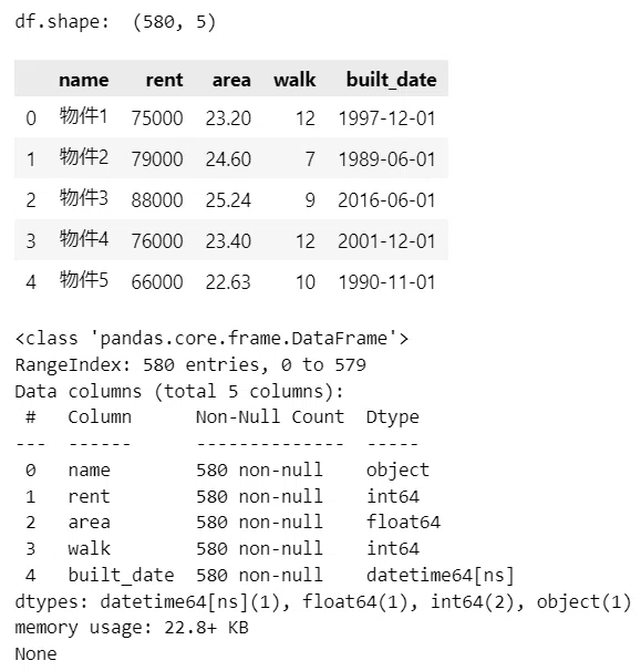
This is property data for 580 items.
There are the following 5 variables.
Note that there are no missing values in any of the variables (580 non-null).

We will process the data.
We will change the date of construction to the number of months since construction (how many months have passed since the building was built).
The reference date for calculating the number of months since construction is tentatively set to "November 2022".
This matches the update date of the article by "TOKYO Restyle".

First, we define a function to calculate the number of months since construction.

### 築年月を築月数に変換する関数の定義
#   pandas.Seriesの日付機能を活用する

def calc_months(x, base_date):
    
    # 基準日（引かれる数）の加工：引数base_dateを文字列から日付型に変換してSeries化
    minuend_date = pd.Series(pd.to_datetime(base_date))
    
    # 築日付（引く数）の加工：引数xをSeries化
    subtrahend_date = pd.Series(x)
    
    # 戻り値：築月数
    #   築月数＝「築日付－基準日」の月数 ※dt.yaerで年、dt.monthで月を取得
    return (minuend_date.dt.year - subtrahend_date.dt.year) * 12 \
            + (minuend_date.dt.month - subtrahend_date.dt.month)

Next, we execute the process to convert it to the number of months since construction.

### 築月数:ageの作成

# データフレームのコピー
data = df.copy()

# 築月数の作成：applyメソッドでcalc_monthsを適用。引数に基準日2022年11月1日を設定
data['age'] = data['built_date'].apply(calc_months, args=('2022-11-01',))

# 築年月built_dateを削除
data = data.drop('built_date', axis=1)

# 先頭５行を表示
display(data.head())

# 加工後のデータフレームをファイルに保存
# data.to_csv('sampledata.csv', index=False, encoding='utf_8_sig')

[Execution Result]

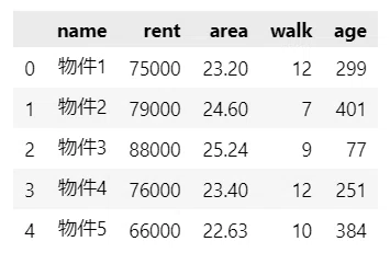
The number of months since construction (age) has been added, and the date of construction (built_date) has been deleted.

Finally, we store the target variable and explanatory variables in a list.
Since we are performing multiple regression analysis to predict rent, the target variable is rent.

### カラム名の取得
# 目的変数
target_col = 'rent'
# 説明変数
feature_cols = data.columns[2:].to_list()
print('feature_cols: ', feature_cols)

[Execution Result]

We stored the names of the three variables, area, walk, and age, in the explanatory variable list feature_cols.

■ When using a processed CSV file
Please download the "Rent Data" CSV file from this link and load the data using the following code.
This CSV file has already been converted to age (number of months since construction).

### csvファイルの読み込み
data = pd.read_csv('./sampledata.csv')

### カラム名の取得
# 目的変数
target_col = 'rent'
# 説明変数
feature_cols = data.columns[2:].to_list()
print('feature_cols: ', feature_cols)

3. Checking the data overview
For now, we will execute pandas describe to check the summary statistics.

### 要約統計量の表示
data.describe()

[Execution Result]

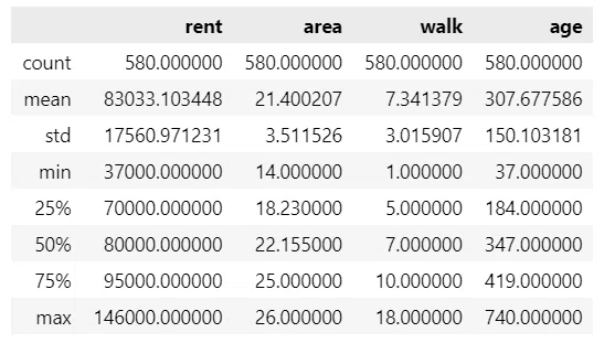
Rent ranges from 37,000 yen to 146,000 yen (median is 80,000 yen), and the age of the building varies from 37 months (about 3 years) to 740 months (over 60 years).

Next, we will check the histograms of the explanatory variables and the scatter plots between each variable.
We will use seaborn's pairplot to draw them all at once.

### ヒストグラムと散布図の描画：seabornのpairplotの利用

sns.pairplot(
    data[feature_cols + [target_col]],    # 描画するデータ
    kind='reg',                           # 回帰直線付き散布図regplotを指定
    corner=True,                          # 行列右上を非表示
    diag_kws={                            # 対角要素の引数
        'ec': 'white'},                   #   ヒストグラムの輪郭線の色     
    plot_kws={                            # 非対角要素の引数
        'ci': None,                       #   回帰直線の信頼区間を非表示
        'scatter_kws': {                  #   散布図の引数
            's': 10,                      #     散布図の点のサイズ
            'alpha': 0.5},                #     散布図の点の透明度
        'line_kws': {                     #   回帰直線の引数
            'color': 'red'},              #     回帰直線の色
        },          
    );

[Execution Result]

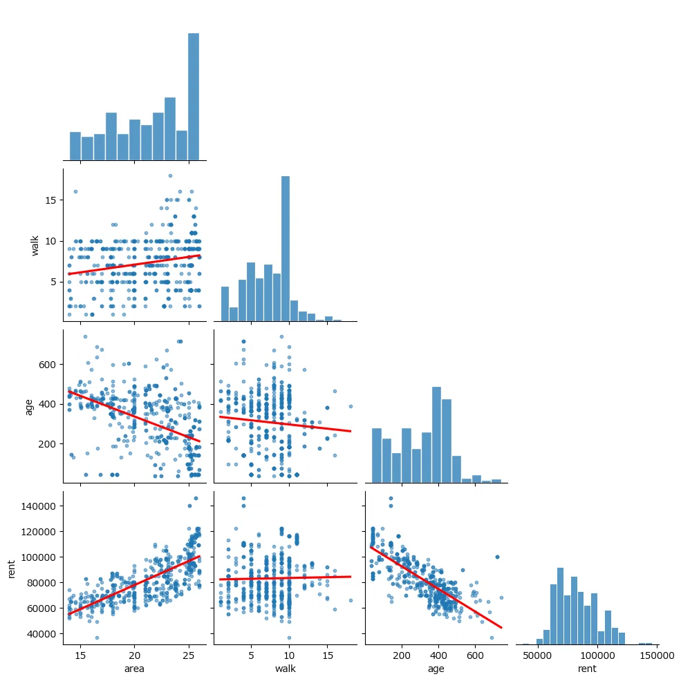
[Impressions of the histogram]
・There are many properties with an area of 25㎡ or more.
　Perhaps those 26㎡ or larger are grouped under "26".
・Rent looks bell-shaped, but 150,000 yen exists as an outlier.

[Impressions of the relationship between explanatory variables and the target variable]
The bottom row contains scatter plots of the explanatory variables and the target variable.
Area seems to have a positive correlation, and building age seems to have a negative correlation.
There seems to be no correlation between walking distance (minutes) and rent.

[Impressions of the relationship between explanatory variables]
・There seems to be a weak negative correlation between area and building age.
　Are newer buildings larger in area...?

Let's check the correlation coefficients.

### 相関行列の表示

# corr関数で相関行列を取得
corr = data.corr(numeric_only=True)
# 相関行列の表示
display(corr)
# 相関行列をヒートマップで可視化
sns.heatmap(data=corr, annot=True);

[Execution Result]

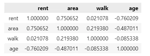
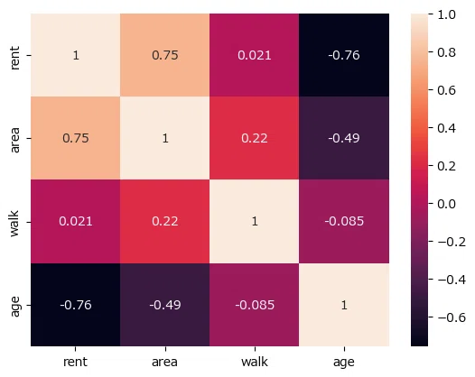
What we observed in the scatter plots has become clear with the numerical values.
There is almost no correlation between walk (walking minutes) and rent.
The walking distance in the data is 1 to 18 minutes.
If it's about an 18-minute walk from Sangen-jaya Station, does it not affect the rent...?

Let's check the partial correlation coefficients.
With partial correlation coefficients, we can see the correlation by removing the influence of other variables.
We will use pingouin's pcorr() to calculate the partial correlation coefficients.

### 偏相関係数の表示
data.iloc[:, 1:].pcorr().round(3)

[Execution Result]

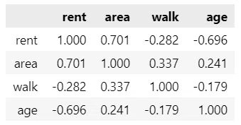
The partial correlation coefficient between walk (walking minutes) and rent is -0.282.
A weak negative correlation has been revealed, where rent becomes cheaper as you get further from the nearest station.
We were able to confirm a correlation that matches our intuition!

I have a feeling that the three explanatory variables are influencing the target variable: rent.

④ Regression Analysis
Let's consider whether it is better to use all three explanatory variables or limit it to fewer variables while looking at the model evaluation metrics.

Let's create linear regression models for all combinations of explanatory variables and obtain the evaluation metrics.
This is a slightly long code.
We are setting up the linear regression model with "sm.OLS(data[target_col], sm.add_constant(data[features])).fit()".

### 説明変数の組み合わせごとに回帰分析を実施して評価指標を取得

## 説明変数の組み合わせをリスト化
#  ・for文を回して組み合わせに入れる説明変数の数（１～３）を指定
#  ・itertoolsのcombinationsで説明変数の数（１～３）ごとの組み合わせを取得

feat_combi_list = []
for num in range(len(feature_cols)):
    for combi in combinations(feature_cols, num+1):
        feat_combi_list.append(list(combi))
print('説明変数の組み合わせ:\n', feat_combi_list)

## 回帰分析の実施
#  ・説明変数の組み合わせごとにstatsmodelsのOLS（線形回帰分析）を実行
#  ・分析結果から自由度調整済み決定係数、RMSE、MAE, AIC, BICを算出してリスト化

adj_R2, rmse, mae, aic, bic = [], [], [], [], []
for features in feat_combi_list:
    # 回帰分析の実行
    results = sm.OLS(data[target_col], sm.add_constant(data[features])).fit()
    # モデルの自由度調整済み決定係数、RMSE、MAE、AIC、BICをリスト化
    adj_R2.append(results.rsquared_adj)
    rmse.append(mean_squared_error(data[target_col], results.fittedvalues,
                                   squared=False))
    mae.append(mean_absolute_error(data[target_col], results.fittedvalues))
    aic.append(results.aic)
    bic.append(results.bic)

## 評価指標をデータフレーム化
result_df = pd.DataFrame({
                          '説明変数': feat_combi_list,
                          'Adj_R2' : adj_R2,
                          'RMSE': rmse,
                          'MAE': mae,
                          'AIC': aic,
                          'BIC': bic,
                         })

## 自由度調整済み決定係数で降順ソートして評価指標を表示
display(result_df.sort_values(by='Adj_R2', ascending=False).round(3))

[Execution Result]
We set up linear regression models for the following seven combinations.

They are listed in descending order of the adjusted R-squared (Adj_R2).

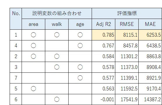
For all evaluation metrics, the model using all three explanatory variables yielded the best results.

From here on, we will examine the multiple regression model using the three explanatory variables.

⑤ Analysis of Multiple Regression Model
We will perform regression analysis using the statsmodels formula API (an R-like API).
By specifying the formula as 'rent ~ area + walk + age', we set three explanatory variables in the regression model.

### ３つの説明変数を用いた回帰分析の実行
results = smf.ols('rent ~ area + walk + age', data=data).fit()

# 回帰式の表示
print(f'回帰式: rent = {results.params.Intercept:.3f} '
      f'{results.params.area:+.3f}*area {results.params.walk:+.3f}*walk '
      f'{results.params.age:+.3f}*age\n')

# 回帰分析の結果の表示
print(results.summary())

【Execution Results】

【Regression Equation】
$${Rent=50620.565+2656.346 \times Area(m^2) -810.902 \times Walk(min) -60.065 \times Age(months)}$$

【Test of Significance of Regression】
The $${p}$$-value of the $${F}$$-statistic (Prob(F-statistic)) is $${0.000 \cdots}$$.
Let's perform a statistical hypothesis test with a significance level of $${5\%}$$.
Since the $${p}$$-value of $${0.000 \cdots}$$ is smaller than the significance level, we can reject the null hypothesis.

【Conclusion】
The null hypothesis is rejected at the $${5\%}$$ significance level, and it can be said that this regression model is significant (at least one of the partial regression coefficients affects the objective variable).

【Test of Significance of Regression Coefficients】
The $${p}$$-value (P > | t |) of the $${t}$$-value for each regression coefficient is $${0.000 \cdots}$$.
Let's perform a statistical hypothesis test with a significance level of $${5\%}$$.
Since the $${p}$$-value of $${0.000 \cdots}$$ is smaller than the significance level, we can reject the null hypothesis.

【Conclusion】
The null hypothesis is rejected at the $${5\%}$$ significance level, and it can be said that all partial regression coefficients are significant (all regression coefficients affect the objective variable).

⑥ Execution of Analysis of Variance
We will perform a one-way analysis of variance using anova_lm from statsmodels.

### 分散分析の実行

# データフレームの表示桁数の設定
pd.options.display.float_format = '{:,.2f}'.format

# 一元配置分散分析の実行 statsmodelsのanova_lmを利用
anova = sm.stats.anova_lm(results, typ=1)
display(anova)

【Execution Results】

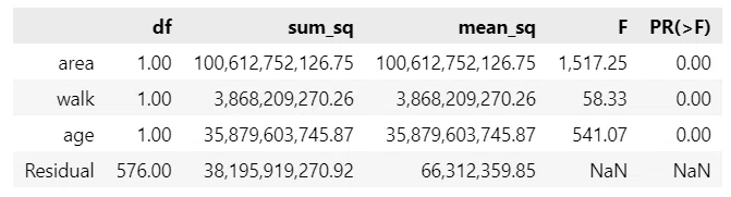
The regression row is displayed broken down by partial regression coefficients.

Let's add the regression row and the total row.

### 「回帰」と「合計」の行を追加した一元配置分散分析表の表示

## 回帰行の編集

# 回帰の自由度の算出
reg_df = anova.loc[['area', 'walk', 'age'], 'df'].sum()

# 回帰のSeriesを作成 ：自由度、平方和、平均平方、F値、p値
regs = pd.Series([reg_df, results.ess, results.mse_model, results.fvalue,
                  results.f_pvalue], 
                 index=anova.columns, name='Regression')

## 合計行の編集

# 合計の自由度と平方和の算出
total_df = anova.loc['Residual', 'df'] + reg_df
total_sum_sq = results.ess + results.ssr

# 合計のSeriesを作成　：自由度、平方和、その他の項目は欠損値
totals = pd.Series([total_df, total_sum_sq, np.nan, np.nan, np.nan],
                   index=anova.columns, name='Total')

## データフレームを統合　1列のみのデータはto_frame().Tで縦のデータフレーム化
anova = pd.concat([anova.iloc[:3, :],               # area～ageの行
                   regs.to_frame().T,               # Regressionの行
                   anova.iloc[3, :].to_frame().T,   # Residualの行
                   totals.to_frame().T],            # Totalの行
                  axis=0)

## 一元配置分散分析表の表示
display(anova)

【Execution Results】

Done!
The bottom three rows correspond to the one-way ANOVA table for the multiple regression model described in the Level 2 textbook.

⑦ Confirmation of Residual Diagnostic Plots
In the statsmodels output, the probabilities in the red box in the figure below are used for testing the assumption of normality of residuals (the assumption that residuals follow a normal distribution).
Since both probabilities are $${0.000 \cdots}$$, it suggests that the residuals do not follow a normal distribution.

Let's check the residual diagnostic plots.
At the same time, let's check the independence of residuals, homoscedasticity of residuals, and outliers.
We will use the lmdiag library.
Install it if necessary.

### 残差診断プロットの描画
# pip install lmdiag

plt.figure(figsize=(12, 12))
lmdiag.plot(results);

【Execution Results】

■ Impact when the assumption of normality of residuals is not met
The judgment of the significance test of the regression using the $${F}$$-value may become inaccurate.
This is because one of the conditions under which the $${F}$$-test statistic can be assumed to follow an $${F}$$-distribution is that the residuals follow a normal distribution.

■ Summary

[Statistical Perspective]
In a statistical context, the opinion would likely be that this linear multiple regression model should be reviewed.
There seem to be solutions such as transforming variables or considering other models, such as adding interaction terms.
Actually, I attempted to build a model by transforming variables using logarithmic transformation, Box-Cox transformation, etc., but I could not ensure the normality of the residuals.
Also, since interaction terms are (likely) outside the scope of the Grade 2 Statistical Test exam, I will stop digging deeper into them here.

[Machine Learning Perspective]
In contexts such as machine learning, it appears that models are evaluated from the perspectives of high prediction accuracy and ease of explanation.
Since the linear regression model ensures ease of explanation, it is thought that the decision on whether to use this multiple regression model will be made based on the prediction accuracy evaluation using the remaining test data.

Download Python sample files
You can download the sample files in Jupyter Notebook format from this link.

Let's create it in EXCEL!

Let's use the "Regression" feature in Data Analysis to perform regression analysis with various combinations of explanatory variables.

Data Overview
Rent data is stored in the "Data" sheet.
It has been converted to age (months since construction).

Regression Analysis Procedure

From the menu, select "Data" > "Data Analysis" to open the "Data Analysis" screen, select "Regression," and click the "OK" button.

In the input range of the "Regression" screen, specify the range of data including the item names. (This corresponds to the red and blue frames.)
Let's check "Labels" and "Residuals."
Select a new worksheet to create a regression analysis sheet.
When you click the "OK" button, the results of the regression analysis will be displayed.

Checking the results of the regression analysis

Here are the regression analysis results for all 7 patterns!

1. Explanatory variables: area, walk, age

2. Explanatory variables: area, walk

3. Explanatory variables: walk, age

4. Explanatory variables: area, age

5. Explanatory variables: area

6. Explanatory variables: walk

7. Explanatory variables: age

■ Summary Table
I have summarized the evaluation indices of the seven regression models in one table.

You may already know this from the Python results, but...
The evaluation metrics for the model using all three explanatory variables yielded the best results across the board.

Let's check the partial regression coefficients of the best model.

[Regression Equation]
$${Rent=50620.56+2656.35 \times Area(m^2) -810.90 \times Walk(min) -60.07 \times Age(months)}$$

■ Test for Significance of Regression Coefficients
The $${p}$$-value for the $${t}$$-value of each regression coefficient is $${0.000 \cdots}$$.
Let's perform a statistical hypothesis test with a significance level of $${5\%}$$.
Since the $${p}$$-value of $${0.000 \cdots}$$ is smaller than the significance level, we can reject the null hypothesis.

[Conclusion]
At a significance level of $${5\%}$$, the null hypothesis is rejected, and it can be said that all partial regression coefficients are significant (all regression coefficients affect the objective variable).

■ One-Way ANOVA Table

■ Test for Significance of Regression
The $${p}$$-value (Significance F) of the $${F}$$-value is $${0.000 \cdots}$$.
Let's perform a statistical hypothesis test with a significance level of $${5\%}$$.
Since the $${p}$$-value of $${0.000 \cdots}$$ is smaller than the significance level, we can reject the null hypothesis.

[Conclusion]
At a significance level of $${5\%}$$, the null hypothesis is rejected, and it can be said that this regression model is significant (at least one of the partial regression coefficients affects the objective variable).

■ How to calculate RMSE and MAE
You can easily calculate RMSE and MAE from the regression analysis results.

① RMSE (Root Mean Square Error)

The blue "Residual Variation" is the sum of squared residuals.
RMSE is the value obtained by dividing the sum of squared residuals by the number of data points (this is MSE: Mean Squared Error) and taking the square root.
In the green box, we are calculating the square root of "Residual Variation" ÷ "Number of Observations".

② MAE (Mean Absolute Error)

MAE is the value obtained by dividing the sum of the absolute values of the residuals by the number of data points.
The residuals are at the bottom of the regression analysis table. It is the blue part.
The absolute value is calculated using the ABS function in EXCEL.
In the green box, we are summing the absolute values of the "residuals" and dividing by the "number of observations".

Download EXCEL Sample File
You can download the EXCEL sample file from this link.

Let's try creating it in R!

We will practice regression analysis using an R script.
The code is very simple.

Download CSV File
You can download the "Rent Data" CSV file from this link.
It has already been converted to age (months).

① Loading Data
Load the CSV file that has already been converted to age (months).

### データの読み込み
data <- read.csv("sampledata.csv")
# データの要約表示
str(data)
summary(data)

[Execution Results]
The overview of data items and summary statistics are displayed.

② Displaying correlation coefficients
Display the correlation matrix.

### 相関係数の計算
cor(data[2:5])

【Execution Results】
The first row displays the correlation coefficients between the target variable 'rent' and the three explanatory variables.
There is a relatively strong correlation between 'rent' and both 'area' and 'age' (number of months since construction).

The basic statistics for both the Central and Pacific leagues have been displayed.
You can check the number of data points (n), mean, standard deviation (sd), median, minimum (min), and maximum (max).
The difference in the mean is $${233.67-185.33=48.34}$$ (ten thousand people).

③ Drawing a correlation matrix
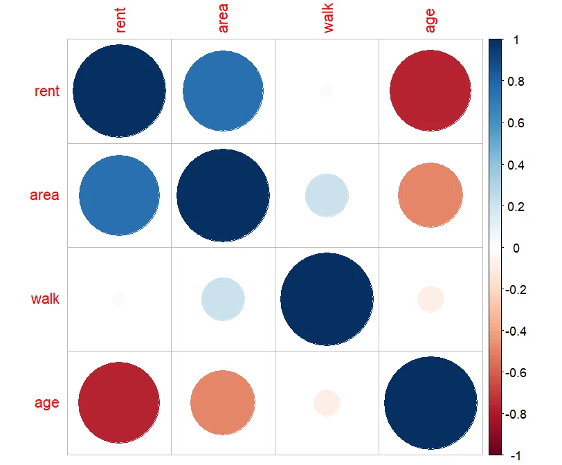
Let's visualize the magnitude of the correlation coefficients using corrplot.

### 相関行列の描画 by corrplot
# install.packages("corrplot")
library(corrplot)
corrplot(cor(data[2:5]))

【Execution Results】
The size of the circles indicates the strength of the correlation, and the color indicates whether the correlation is positive or negative.
There seems to be some correlation between 'area' and 'age'.

④ Drawing a scatter plot matrix
Let's visualize the relationships between variables by drawing scatter plots using psych.

### 散布図行列の描画 by psych
# install.packages("psych")
library(psych)
psych::pairs.panels(data[, seq(2, 5)])

【Execution Results】
Let's look at the 'rent' column on the far left.
It is clear that 'area' and 'age' have a correlation with 'rent'.
Also, the histograms for each variable show that the distribution of 'area' is skewed toward larger sizes, 'walk' (minutes to station) is skewed toward being closer to the station, and 'age' is skewed toward newer buildings.

⑤ Executing regression analysis
The main event is here.
The part 'lm(rent ~ area + walk + age, data=data)' uses almost the same syntax as the formula API in Python's statsmodels.

### 回帰分析の実施と結果表示
data.lm <- lm(rent ~ area + walk + age, data=data)
summary(data.lm)

【Execution Results】
This is the 'statistical software output' familiar from Statistical Test questions!

【Test of Regression Significance】
The $${p}$$-value for the $${F}$$-statistic is $${0.000 \cdots}$$.
Let's conduct a statistical hypothesis test with a significance level of $${5\%}$$.
Since the $${p}$$-value of $${0.000 \cdots}$$ is smaller than the significance level, we can reject the null hypothesis.

【Conclusion】
The null hypothesis is rejected at the $${5\%}$$ significance level, and we can say that this regression model is significant (at least one of the partial regression coefficients affects the target variable).

【Test of Significance of Regression Coefficients】
The $${p}$$-value (Pr(>| t |)) for the $${t}$$-statistic of each regression coefficient is $${0.000 \cdots}$$.
Let's conduct a statistical hypothesis test with a significance level of $${5\%}$$.
Since the $${p}$$-value of $${0.000 \cdots}$$ is smaller than the significance level, we can reject the null hypothesis.

【Conclusion】
The null hypothesis is rejected at the $${5\%}$$ significance level, and we can say that all partial regression coefficients are significant (all regression coefficients affect the target variable).

⑥ Executing analysis of variance
This is the final code.
We load the regression analysis result 'data.lm' and execute 'anova'.

### 分散分析の実施と結果表示
anova(data.lm)

【Execution Results】
The analysis of variance table has been displayed.

Downloading R sample files
You can download the sample file in R script format from this link.

This concludes the multiple regression analysis and analysis of variance for this article.
Thank you very much for staying with me until the final episode.

Conclusion

We have solved all the problems by field and item from the 'Statistical Test Grade 2 Official Problem Collection - CBT Compatible Version'.
Thank you very much for joining me on this long journey.

Those who continued the journey with me have surely experienced the basics of statistics and touched upon its interest and importance.
I sincerely hope that a statistical perspective will be useful in your lives going forward.
Please feel free to return to these articles anytime.

Keep on 'Relaxed Statistics'!

Thank you for reading until the end.
Goodbye.

Articles in the Relaxed Statistics Series

Next article

Previous article

Table of contents