Bayesian Modeling for Chapter 14 "When Will I Write the Manuscript?" in PyMC Ver. 5

This article is a statistical documentary depicting the process of "experimentally" implementing the Bayesian model from Chapter 14, "When Will I Write the Manuscript?" of the text "Fun Bayesian Modeling" using PyMC Ver. 5. In this chapter, the author, who struggles with slow writing, codes and accumulates "daily writing volume data" for seven manuscripts, and

infers when the writing volume accelerated using a "change-point detection model".

This time, I created a "model different from the text" and worked on the inference for the seven manuscripts, and was able to obtain inference results close to the text for about half of them!

When will the author's motivation switch finally turn ON?
Let's model it with PyMC and enjoy Bayesian statistics!

Please refer to the linked article for the introduction of the text, citation notation, series preface, and version information for PyMC, etc.

The data used in the text, along with sample scripts for R, Stan, etc., can be obtained by downloading them from the publisher's website.

Summary

Overview of the text

Author: Dr. Yoshihiko Kunisato
Model Difficulty: ★★★.. (Average)

Self-Evaluation

Rating

$$
\begin{array}{c:c:c}
Implementation Accuracy & ★★★..& Decent \\
Result Reproducibility & ★★★..& Decent \\
Fun Factor & ★★★★★& Fun! \\
\end{array}
$$

Evaluation Points

• When using whether it matches the change point in the text (number of days elapsed since the start of writing) as an evaluation axis, the match rate was 4/7, meaning more than half of the manuscripts matched. However, out of the three manuscripts that did not match, two failed to converge.
  

Ingenuity, Joy, and Reflections

• In Stan, which cannot have discrete values as parameters, we deal with this using a method called "marginalization," but since PyMC can handle discrete values, we can build a model different from Stan. This time, I incorporated discrete value parameters into the model. The reason is that I do not know how to perform "marginalization" using PyMC. I want to master the method of marginalization (taking the sum of probabilities) someday.
  

  
  
  

Model Overview

Overview of the text's research and experiments

■ Monitoring Writing Volume and Change Points
The author, who belongs to the group that struggles to make progress on papers and manuscripts, reportedly read the following book.

There are two main points.
・Creating and adhering to a writing schedule
・Monitoring writing volume

What is impressive about the author is that they automated the management of their writing volume.
It seems that when writing in Google Docs, Google Apps Script automatically records the writing volume in a Google Spreadsheet and even sends automated email notifications about progress.
Please check the author's website here for the detailed method.

If you thoroughly implement such enthusiastic visualization of writing volume and plan-versus-actual management,you would expect that writing would proceed at an incredible pace from the very beginning, but there is also the possibility that "truth is stranger than fiction" (how exciting).

■ Overview of the Experiment
The "writing volume data for seven manuscripts" from the author's own manuscript creation work is the star of this Bayesian modeling.
It is that very data that led the author to say, "Data is sometimes cruel."

Modeling the Text

■ Objective Variable and Parameters of Interest
The objective variable ${text_{day}}$ is the daily cumulative writing volume (number of characters).
The parameter of most interest is ${cp}$, which is the change point (number of days) where the writing volume accelerated.

■ Model
The first formula (or rather, programming code) shows the cumulative writing volume "before the change point," and the second formula shows the cumulative writing volume "after the change point."
Both are models that follow a normal distribution where the mean parameter is the cumulative writing volume of the previous day plus either ${\mu_1}$ (writing volume per day before the change point) or ${\mu_2}$ (writing volume per day after the change point).

In the implementation using Stan, it is said that the change point ${cp}$, which takes discrete integer values, cannot be estimated directly as a parameter, so a method called marginalization is used to estimate the change point ${cp}$.
I am not very familiar with the marginalization method, so I will not touch upon it in this article.

■ Analysis and Analysis Results
I believe the descriptions in the text regarding the analysis method and analysis figures are accurate, so I recommend reading the text.
For the analysis results using PyMC modeling, please see the [5. Analysis] section in the "PyMC Implementation" chapter.

PyMC Implementation

Let's enjoy PyMC & Python !

Preparation and Data Confirmation

1. Import

### インポート

# ユーティリティ
import pickle

# 数値・確率計算
import pandas as pd
import numpy as np

# PyMC
import pymc as pm
import pytensor.tensor as pt
import arviz as az

# 描画
import matplotlib.pyplot as plt
import seaborn as sns
plt.rcParams['font.family'] = 'Meiryo'

# ワーニング表示の抑制
import warnings
warnings.simplefilter('ignore')

2. Loading Data
Load the csv file into a pandas DataFrame.

### データの読み込み

# データの読み込み
data = pd.read_csv('data.csv')

# データの表示
display(data)

[Execution Results]
There are 123 rows and 8 columns in total.
The data items are as follows:
day: Days elapsed since writing started (1 to 123 days)
draft_1 to draft_7: Cumulative writing volume (number of characters) for manuscripts 1 through 7 at the time of elapsed days

3. Data Overview and Statistics

First, let's check the summary statistics.

### 要約統計量の表示
data.describe().round(2)

[Execution Result]
When 75% of the days have passed, most manuscripts have not even reached 50% of completion (what is monitoring?).

Following the text, let's plot the cumulative writing amount by elapsed days.
This corresponds to Figure 14.2 in the text.

### 各原稿の執筆状況 ★図14.2に対応

plt.figure(figsize=(10, 10))
# 原稿１～７まで繰り返し処理
for i, col in enumerate(data.columns[1:]):
    # サブプロットの作成
    ax = plt.subplot(4, 2, i+1)
    # 点グラフの描画
    ax.plot(data['day'], data[col], 'o', markersize=2)
    # タイトル（原稿ｎ）の表示
    ax.set_title(f'原稿{i+1}')
# 修飾
plt.suptitle('経過日数と各原稿の累積執筆量(字数)', fontsize=16)
plt.tight_layout()
plt.show()

[Execution Result]
W-well, this is... (what is schedule management?).
Conversely, maybe they have the constitution to write it easily if they have 10 days!?

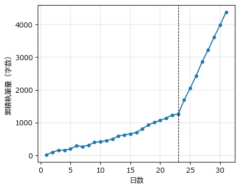
4. Simulation of the Change Point Detection Model
Following the text, we will perform a simulation of the change point detection model.
This corresponds to Figure 14.3 in the text.
Since the random seed is different from the text, the simulation results differ from the text.

### 変化点検出モデルのシミュレーション ★図14.3に相当

# 設定
days, cp = 31, 23                  # 日数、変化点
mu1, mu2, sigma = 50, 400, 30      # 変化点前の平均、変化点後の平均、標準偏差

# 初期値
text = np.zeros(days)
np.random.seed(123)

# シミュレーションの実施
for i in range(days):
    if i==0:
        text[i] = np.random.normal(loc=mu1, scale=sigma, size=1)
    elif i <= cp-1:
        text[i] = np.random.normal(loc=text[i-1] + mu1, scale=sigma, size=1)
    else:
        text[i] = np.random.normal(loc=text[i-1] + mu2, scale=sigma, size=1)

# 描画
plt.figure(figsize=(5, 4))
plt.plot(range(1, days+1), text, 'o-', markersize=4)
plt.axvline(cp, color='black', lw=0.8, ls='--')
plt.xlabel('日数')
plt.ylabel('累積執筆量（字数）')
plt.grid(lw=0.3)
plt.show();

[Execution Result]
You can feel that the writing is accelerating after day 23, which is the change point $${cp}$$.
The model we are tackling with PyMC is exactly about exploring change points like this graph!

Model Construction

Mathematical Expression of the Model
PyMC's MCMC can handle discrete parameters.
Therefore, in this article, we use a model where the change point $${cp}$$ follows a DiscreteUniform distribution.
This is a "pseudo-mathematical" notation that mixes in the atmosphere of the PyMC model we want to aim for.

$$
\begin{align*}
\mu_1 &\sim \text{Uniform}\ (\text{lower}=-100000,\ \text{upper}=100000) \\
\mu_2 &\sim \text{Uniform}\ (\text{lower}=-100000,\ \text{upper}=100000) \\ \sigma &\sim \text{HalfCaushy}\ (\text{beta}=100) \\
cp &\sim \text{DiscreteUniform}\ (\text{lower}=1,\ \text{upper}=123) \\
\text{if}\ &dayIdx==0: \\
&\quad \mu = \mu_1 \\
\text{elif}\ &dayIdx \leq cp-1: \\
&\quad \mu = text_{day - 1} + \mu_1 \\
\text{elif}\ &dayIdx > cp-1: \\
&\quad \mu = text_{day - 1} + \mu_2 \\
text_{day} &\sim \text{Normal}\ (\text{mu}=\mu,\ \text{sigma}=\sigma) \\
\end{align*}
$$

1. Model Definition
Create a date index by subtracting 1 from the date day of the data.

### 日付インデックスday-1の作成
day_idx = data['day'].values - 1

Note that in the text, the cumulative writing amount is divided by 1000 for Stan processing, but in this article, we do not divide by 1000.

Next, we move on to the model definition.
This time, since we are "building almost the same model separately for each of the seven manuscripts," we will functionalize the process from model definition to MCMC execution to posterior predictive sampling, and call the function for each manuscript.

### MCMC実行関数１　正規分布モデル

def exec_mcmc1(draft_col, disp=False):

    with pm.Model() as model1:
        
        ### データ関連定義
        # coordの定義
        model1.add_coord('data', values=data.index, mutable=True)
        # dataの定義
        text = pm.ConstantData('text', value=data[draft_col].values,
                               dims='data')
        dayIdx = pm.ConstantData('dayIdx', value=day_idx, dims='data')

        ### 事前分布
        mu1 = pm.Uniform('mu1', lower=-100000, upper=100000)
        mu2 = pm.Uniform('mu2', lower=-100000, upper=100000)
        sigma = pm.Uniform('sigma', lower=0, upper=100000)
        cp = pm.DiscreteUniform('cp', lower=1, upper=data['day'].max())
        
        ### muの計算
        mu = pt.switch(pt.eq(dayIdx, 0), mu1, 
                       pt.switch(pt.le(dayIdx, cp-1),
                                 text[dayIdx-1] + mu1, text[dayIdx-1] + mu2))
            
        ### 尤度    
        likelihood = pm.Normal('likelihood', mu=mu, sigma=sigma, observed=text,
                               dims='data')
        
        ### モデルの表示・可視化　disp引数＝Trueの場合に実行
        if disp:
            display(model1)            
            display(pm.model_to_graphviz(model1))
        
        ### 事後分布からのサンプリング
        idata1 = pm.sample(draws=5000, tune=25000, chains=4, target_accept=0.95,
                           random_seed=1234)

        ### 事後予測サンプリング
        idata1.extend(pm.sample_posterior_predictive(idata1))
    
    return idata1

[Structure of Function Processing]
1. PyMC model definition: Data-related definitions to likelihood
2. Model display: Display and visualization of the model
3. Sampling from the posterior distribution
4. Posterior predictive sampling

[Model Annotations]

• Definition of coords
  You can name coordinates and set the values those coordinates can take.
  This time, I set the following one:
  - Row coordinate: Name "data", value "row index"

• Definition of data
  I set the objective variable $${text}$$ and the date index $${dayIdx}$$.

• Prior distribution of parameters

  • $${\mu_1}$$ and $${\mu_2}$$ are set to a continuous uniform distribution taking the range $${[-100000, 100000]}$$.In the text, they are set to $${[-100, 100]}$$; however, since the cumulative writing amount is not divided by 1000 in this article, I multiplied the range of the continuous uniform distribution by 1000.

  • Similarly, $${\sigma}$$ is a continuous uniform distribution taking the range $${[0, 100000]}$$.

  • The change point $${cp}$$ is a discrete uniform distribution taking the range of elapsed days $${[1, 123]}$$.

• Calculation of mu
  When the elapsed days are less than or equal to the change point, $${\mu_1}$$ is added to the previous day's cumulative writing amount, and when it exceeds the change point, $${\mu_2}$$ is added to the previous day's cumulative writing amount.

• Likelihood
  It follows a normal distribution with $${\mu}$$ and $${\sigma}$$ as parameters.

[Sampling the Posterior Distribution]
Since there are parameters following discrete distributions, the NUTS sampler uses the standard PyMC sampler.
Processing time increases compared to using numpyro.
Additionally, because tune (burn-in period) has been increased to 25,000 (the text uses 500), this is a factor contributing to the longer processing time.

2. Execution of MCMC function
We will infer all seven manuscripts at once using a for-loop.
The processing time is approximately 36 minutes.

### 事後分布＆事後予測サンプリングの実施　尤度：正規分布　36分

# 原稿１～７までの推論データを格納するリストの初期化
idata1 = []
# 原稿１～７まで繰り返し処理
for i, col in enumerate(data.columns[1:]):
    # 原稿の番号を表示
    print(f'--- {i+1} ---')
    disp = False
    # 原稿１のとき、PyMCモデルを可視化
    if i==0:
        disp = True
    # 事後分布＆事後予測のサンプリングを実施、リストに推論データを格納
    idata1.append(exec_mcmc1(col, disp=disp))

[Execution Result 1: Model Display and Visualization]
This is a relatively simple model.
The same type of model is applied to all seven manuscripts.
Since the model is redefined for each manuscript, the inferred values are calculated for each manuscript individually.

[Execution Result 2: MCMC and Posterior Prediction]
These are manuscripts 1 to 3.

These are manuscripts 4 to 6.

This is manuscript 7.

Manuscript 6 seems to have a long processing time and a high number of divergent data points.
The text and R code mention manuscript 6 (the range of cp is wide, estimation takes time), so there might be something peculiar about manuscript 6.

3. Confirmation of sampling data
We will check the R-hat and trace plots.
The convergence check for the posterior distribution is set to R-hat <= 1.1.

### r_hat>1.1の確認

# 原稿１～７まで繰り返し処理
for i in range(len(idata1)):
    # 原稿の番号を表示
    print(f'--- {i+1} ---')
    # R_hatの算出
    rhat_idata = az.rhat(idata1[i].posterior)
    # R_hat > 1.1となる変数の数を表示
    display((rhat_idata > 1.1).sum())

[Execution Result]
The parameters for manuscripts 2 and 5 have R-hat > 1.1, meaning they have not converged.
For cases like manuscripts 2 and 5 where the manuscript is written "gradually," model improvement might be necessary.

Please note that from here on, when using the data, manuscripts 2 and 5 cannot be formally analyzed and should be treated as reference values.

These are the summary statistics of the inferred data.

### 推論データの要約統計量の表示

# 原稿１～７まで繰り返し処理
for i in range(len(idata1)):
    # 原稿の番号を表示
    print(f'--- {i+1} ---')
    # 推論データの要約統計量の表示
    display(pm.summary(idata1[i], hdi_prob=0.95))

[Execution Result]
We focus on the mean value of cp.
When rounding to the nearest integer, the "change points" that match those listed in Table 14.2 of the text are manuscripts 1, 3, 4, and 7.
For manuscript 6, out of 6,016 total characters, writing 3,800 characters all at once in 93 days may have led to the instability in the inferred values. The 95% HDI of mu2 has become an impossible value of [-91111, 97075].
Manuscript 6 might not be compatible with this model.

These are the trace plots.

### トレースプロットの描画

# 原稿１～７まで繰り返し処理
for i in range(len(idata1)):
    # 原稿の番号を表示
    print(f'--- {i+1} ---')
    # トレースプロットの描画
    pm.plot_trace(idata1[i], figsize=(10, 6))
    plt.tight_layout()
    plt.show()

[Execution Result]
Manuscript 1:
It feels like a strong assertion that the change point is 121 days!
It resulted in a clean plot.

Manuscript 2:
The four chains are split into two distributions.

Manuscript 3:
The change point is almost exactly 119 days!

Manuscript 4:
The change point is 117 days!

Manuscript 5:
The distribution is split into two.

Manuscript 6:
Barcode patterns indicating divergence are scattered throughout.
The centers of the distributions seem to match across the four chains.

Manuscript 7:
The change point is almost exactly 119 days!

5. Analysis
We will plot the writing progress of each manuscript with the change points added, corresponding to Figure 14.4 in the text.
We are using the posterior predictive values of the objective variable (text).

### 変化点を追加した各原稿の執筆状況 ★図14.4に対応

plt.figure(figsize=(10, 10))

for i in range(len(idata1)):
    ## 変化点の平均の算出
    cp_mean = idata1[i].posterior.cp.mean().values
    # 95%HDI区間の算出
    hdi95 = (az.hdi(idata1[i].posterior_predictive, hdi_prob=0.95)
             .likelihood.data)
    ## 描画
    ax = plt.subplot(4, 2, i+1)
    # 95%HDIの描画
    ax.fill_between(x=data['day'], y1=hdi95[:, 0], y2=hdi95[:, 1],
                    color='tomato', alpha=0.4)
    # 事後予測の平均値の描画
    ax.plot(data['day'], 
            (idata1[i].posterior_predictive.likelihood.data.reshape(20000, 123)
            .mean(axis=0)))
    # 観測値の描画
    ax.plot(data['day'], data.iloc[:, i+1], 'o', markersize=1, color='blue')
    # 変化点の描画
    ax.axvline(cp_mean, color='black', lw=0.8, ls='--')
    # 修飾
    ax.set_title(f'原稿 {i+1}: 変化点{cp_mean:.0f}日')
plt.tight_layout()
plt.show()

[Execution Results]
The blue dots are observed values, the blue line is the mean of the posterior predictive values, the red band is the 95% HDI of the posterior predictive values, and the black vertical dotted line is the change point.
The posterior prediction seems to be working well.

[Analysis]

■ Point 1: Suitability of the single change point model
① Change points for manuscripts 1, 3, 4, and 7
Since there is only one point where the amount of writing increases rapidly, it feels easy to represent (and fit) with a single change point model.
② Manuscript 6
There are three stages of change points around 70, 90, and 120 days, so it feels like it cannot be fully represented by a single change point model.
③ Manuscripts 2 and 5
Multi-stage change points can also be observed here.
The model not fitting might be the main reason for the lack of convergence.
(Why was the text able to converge???)

■ Point 2: Thoughts on the timing of changes in writing volume
In the flow of conducting research/experiments, organizing and analyzing data, and writing papers, it feels like standard procedure for the actual writing of the paper to come in the latter half.
On the other hand, if the writing materials are almost all ready and only the drafting and polishing remain, a style of finishing in the last few days out of 123 days could be seen as exposing a lack of planning.
I suspect the author is likely the former.
After all, they are someone who was able to build a system for managing writing volume systematically, even going so far as to write the code for it.

6. Saving inference data (idata)
Let's save it to a file in case you need to reuse the inference data.
Save idata using pickle.

### idata1の保存 pickle
file = r'idata1_ch14.pkl'
with open(file, 'wb') as f:
    pickle.dump(idata1, f)

The code for loading is as follows.

### idataの読み込み pickle
file = r'idata1_ch14.pkl'
with open(file, 'rb') as f:
    idata1_load = pickle.load(f)

This concludes Chapter 13.
Table 14.3, Figure 14.5, and Figure 14.6 have been omitted.

Bonus

I will try the change point detection model familiar from the book "Bayesian Methods for Hackers" (Probabilistic Programming and Bayesian Methods for Hackers).
This book contains abundant examples of Bayesian inference using PyMC and is a recommended volume for making Bayesian methods accessible.

I will start with the conclusion.
・Manuscript 1 did not converge.
・It became a model that easily picks up the first change point.

In the model, the observed values follow a Poisson distribution.
The mean parameter λ of the Poisson distribution differs before and after the change point cp.
The mean parameter λ follows an exponential distribution.

I will share the image of the model.

1. Definition of MCMC execution function

### MCMC実行関数２ ポアソン分布モデル

def exec_mcmc2(draft_col, disp=False):

    with pm.Model() as model2:
        
        # 初日の執筆量の最小値の逆数
        alpha1 = 1 / data.iloc[0, 1:].min()
        # １原稿の最大執筆量の逆数
        alpha2 = 1 / data.iloc[:, 1:].max().max()
        
        ### データ関連定義
        # coordの定義
        model2.add_coord('data', values=data.index, mutable=True)
        # dataの定義
        text = pm.ConstantData('text', value=data[draft_col].values,
                               dims='data')
        dayIdx = pm.ConstantData('dayIdx', value=day_idx, dims='data')

        ### 事前分布
        lam1 = pm.Exponential('lam1', lam=alpha1)
        lam2 = pm.Exponential('lam2', lam=alpha2)
        cp = pm.DiscreteUniform('cp', lower=1, upper=data['day'].max())
        
        ### muの計算
        mu = pt.switch(pt.eq(dayIdx, 0), lam1, 
                       pt.switch(pt.le(dayIdx, cp-1),
                                 text[dayIdx-1] + lam1, text[dayIdx-1] + lam2))
            
        ### 尤度    
        likelihood = pm.Poisson('likelihood', mu=mu, observed=text, dims='data')
        
        ### モデルの表示・可視化　disp引数＝Trueの場合に実行
        if disp:
            display(model2)
            display(pm.model_to_graphviz(model2))

        ### 事後分布からのサンプリング
        idata2 = pm.sample(draws=5000, tune=25000, chains=4, target_accept=0.95,
                           random_seed=1234)
        
        ### 事後予測サンプリング
        idata2.extend(pm.sample_posterior_predictive(idata2))
    
    return idata2

2. Execution of MCMC, etc.
The processing time is approximately 24 minutes and 35 seconds.

### 事後分布＆事後予測サンプリングの実施　尤度：ポアソン分布　24分35秒

# 原稿１～７までの推論データを格納するリストの初期化
idata2 = []
# 原稿１～７まで繰り返し処理
for i, col in enumerate(data.columns[1:]):
    # 原稿の番号を表示
    print(f'--- {i+1} ---')
    disp = False
    # 原稿１のとき、PyMCモデルを可視化
    if i==0:
        disp = True
    # 事後分布＆事後予測のサンプリングを実施、リストに推論データを格納
    idata2.append(exec_mcmc2(col, disp=disp))

[Execution Results] Omitted

3. Confirmation of sampling data
First, let's check for convergence.

### r_hat>1.1の確認

# 原稿１～７まで繰り返し処理
for i in range(len(idata2)):
    # 原稿の番号を表示
    print(f'--- {i+1} ---')
    # R_hatの算出
    rhat_idata = az.rhat(idata2[i].posterior)
    # R_hat > 1.1となる変数の数を表示
    display((rhat_idata > 1.1).sum())

[Execution Results] Only Manuscript 1 is shown
Manuscript 1 did not converge.

Next is the display of summary statistics.

### 推論データの要約統計量の表示

# 原稿１～７まで繰り返し処理
for i in range(len(idata2)):
    # 原稿の番号を表示
    print(f'--- {i+1} ---')
    # 推論データの要約統計量の表示
    display(pm.summary(idata2[i], hdi_prob=0.95))

[Execution Results]
It is puzzling that for some manuscripts, the mean parameter lam1 before the change point cp is larger than lam2 after cp.

Checking the trace plot.

### トレースプロットの描画

# 原稿１～７まで繰り返し処理
for i in range(len(idata2)):
    # 原稿の番号の表示
    print(f'--- {i+1} ---')
    # トレースプロットの描画
    pm.plot_trace(idata2[i], figsize=(10, 6))
    plt.tight_layout()
    plt.show()

[Execution Results]
Manuscript 1:

Manuscript 2:

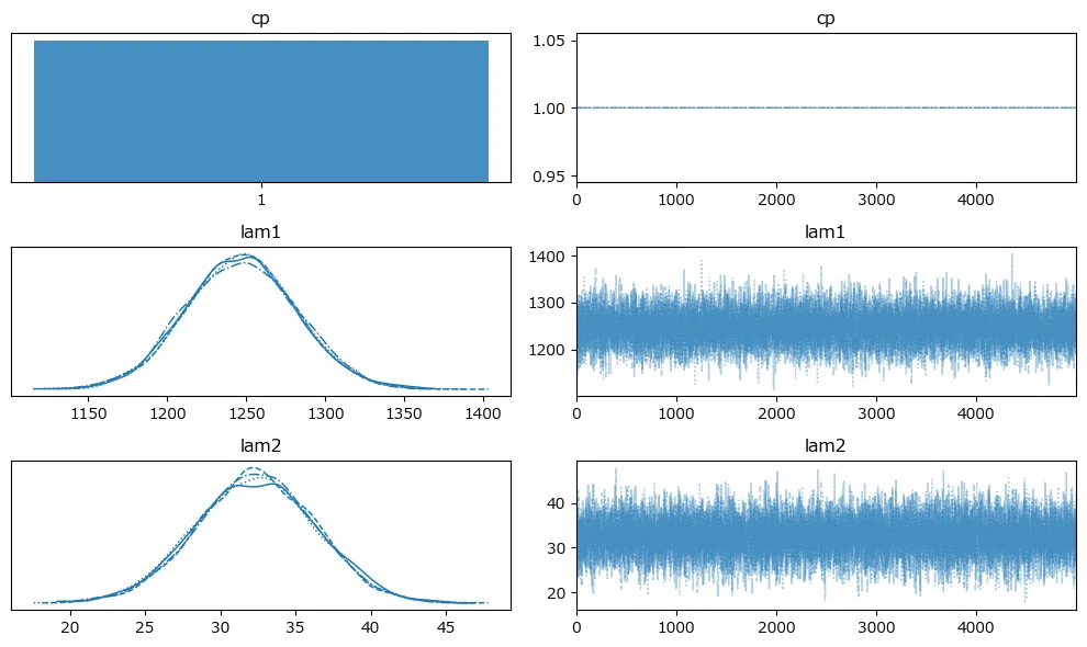
Manuscript 3:

Manuscript 4:

Manuscript 5:

Manuscript 6:

Manuscript 7:

4. Analysis
Now, finally, let's plot the writing progress of the manuscript with the change point added.

### 変化点を追加した各原稿の執筆状況 ★図14.4に対応

plt.figure(figsize=(10, 10))

for i in range(len(idata2)):
    ## 変化点の平均の算出
    cp_mean = idata2[i].posterior.cp.mean().values
    # 95%HDI区間の算出
    hdi95 = (az.hdi(idata2[i].posterior_predictive, hdi_prob=0.95)
             .likelihood.data)
    ## 描画
    ax = plt.subplot(4, 2, i+1)
    # 95%HDIの描画
    ax.fill_between(x=data['day'], y1=hdi95[:, 0], y2=hdi95[:, 1],
                    color='tomato', alpha=0.9, label='事後分布95%HDI')
    # 事後予測の平均値の描画
    ax.plot(data['day'], 
            (idata2[i].posterior_predictive.likelihood.data.reshape(20000, 123)
            .mean(axis=0)))
    # 観測値の描画
    ax.plot(data['day'], data.iloc[:, i+1], 'o', markersize=1, color='blue')
    # 変化点の描画
    ax.axvline(cp_mean, color='black', lw=0.8, ls='--')
    # 修飾
    ax.set_title(f'原稿 {i+1}: 変化点{cp_mean:.0f}日')
plt.tight_layout()
plt.show()

[Execution Results/Analysis-like Inference]
This model seems to agilely scoop up the "signs of subtle changes in writing volume."
It might even be elevated to a premium model that detects the perfect timing for the motivation switch to turn ON = the omen.!!!!
Manuscript 2 is full turbo from day one! (There might have been a parallel world where that happened)

Even so, it's amazing that the inference shows the width of the red band indicating the 95% HDI is super narrow, meaning it's almost the mean value.

That's all for the bonus model.

Conclusion

Writing a Blog Manuscript

In tackling the model for Chapter 14, I looked back on my own attitude toward writing blog manuscripts.

• Deadlines
  Since it's not work or an official task, deadlines are practically non-existent lol
  I do intend to post at a pace of once a week, so by disciplining myself, I can make the concept of a deadline manifest.

• Planning
  There is no plan! I haven't created schedules, WBS, etc., and I don't track actual results or manage progress.
  Being able to write freely as I please is the real thrill of a personal blog ヽ(=´▽`=)ﾉ

• Management
  I don't manage it (I declare! Seriously!).
  Because it's a fun hobby, I can keep writing happily every day!
  I do have a guideline, though. It's to keep a stock of 4 to 5 posts.

• Source of Fun
  It's just writing the results of happily learning text on my blog.
  And rather than saying writing the blog is fun, learning is what's fun (Hobby: Learning).
  Also, I aspire to an environment where I can get the technical information and hints I want via Web search in Japanese.
  I would be happy if my rare (sometimes failed) blog posts could be of use to someone looking for a niche 🍀

Series Articles

Next article

Previous article

Table of Contents

Blog Introduction

I am writing four series of articles on note. Please feel free to take a look!

1. Relaxed Statistics
This is a blog that roughly explores probability and statistics using the Statistical Test Grade 2 problem collection as a guide.
Feel free to read it like a casual conversation. Please do take a look.
It corresponds to the Statistical Test Grade 2 Official Problem Collection CBT Version.

2. Introduction to Time Series Analysis for Psychology with R and Stan, using Python and PyMC Ver. 5
I am working on the time series analysis topics from the book 'Introduction to Time Series Analysis for Psychology with R and Stan' using Python and PyMC Ver. 5.
I believe that practicing with a wealth of themes (topics) will help build fundamental strength in Python and PyMC.
Every day, I work hard at web searches, understanding time series models, grasping Python packages, and translating R/Stan code!
I hope this series will be a useful reference for beginners in Python time series analysis. 🍀

3. Python Machine Learning Programming Practice Log
I have written articles about my various thoughts while studying the book 'Python Machine Learning Programming: PyTorch & scikit-learn Edition'.
This book is a textbook for scikit-learn and PyTorch.
Please feel free to give it a try.

4. Writing about Data Science-ish Things
I write columns on statistics, data analysis, AI, machine learning, and Python on an irregular basis.
Series on 'Statistics', 'Python', 'Mathematics and Python', and 'R' have been created.
Practical records of Bayesian books are also posted.

Thank you very much for reading until the end.