
Drawing the Mandelbrot Set in Processing

Hello, this is 108Hassium.
I have written several articles introducing my own fractal generation programs, but I realized that I have only been discussing advanced topics and have not covered the basics.
※☟Past articles
Therefore, in this article, I will explain from the basics how to draw fractal figures in Processing, using the Mandelbrot set as an example.
※I will explain this assuming you have not read my past articles, but I assume you have already learned the syntax of Processing.
Definition and Calculation Method
First, I will explain the definition of the Mandelbrot set and the calculation method when implemented in a program.
The Mandelbrot set is the set of complex numbers $${c}$$ for which the following sequence does not diverge to infinity.
$${z_0=0}$$
$${z_{n+1}=z_n^2+c}$$
※I have used a different definition in other articles I have written, and the one above is called the "Mandelbrot set of $${z^2+c}$$". The definition in my other articles is more convenient, but since this definition seems to be the formal one, I will use this one in this article.
Using this sequence, you can draw (an approximation of) the Mandelbrot set by following the steps below.
Determine the range on the complex plane you want to draw. (If you set the real and imaginary parts to the range of -2 to 2, the entire Mandelbrot set will fit perfectly.)
Divide the drawing range into a grid.
Pick one complex number from within each grid cell (the corners are fine too), and use that value as $${c}$$ to calculate $${z_n}$$.
Color-code the grid cells based on whether $${z_n}$$ diverged to infinity or not.

It seems that Processing cannot calculate complex numbers directly, so when calculating $${z_n}$$, I will separate it into real and imaginary parts and reduce it to real number calculations.
If we let $${z_n=x_n+y_ni}$$ and $${c=a+bi}$$, the real and imaginary parts of $${z_{n+1}}$$ can be calculated as follows.
$${\begin{cases}x_{n+1}=x_n^2-y_n^2+a\\y_{n+1}=2x_ny_n+b\end{cases}}$$
Whether $${\displaystyle{\lim_{n→\infty}}z_n}$$ diverges to infinity can be determined by the following theorem.
If there exists an $${m}$$ that satisfies $${|z_m|>2}$$, then $${\displaystyle{\lim_{n→\infty}}z_n}$$ will always diverge to infinity.
*The proof is omitted.
Since $${|z_n|=\sqrt{x_n^2+y_n^2}}$$, in practice, you can calculate $${x_n}$$ and $${y_n}$$ one term at a time and determine that it diverges if $${x_n^2+y_n^2}$$ exceeds 4 even once.
However, since the magnitude of $${m}$$ that satisfies $${|z_m|>2}$$ can be arbitrarily large depending on the value of $${c}$$, when performing actual calculations, you should set an appropriate upper limit for the number of iterations and assume it has converged if that limit is reached.
Summarizing the above, the Mandelbrot set can be drawn using the following procedure.
Determine the range on the complex plane you wish to draw.
Divide the drawing area into a grid.
Set an upper limit for the number of iterations.
Pick one complex number from within each grid cell, set that value as $${a+bi}$$, and calculate $${x_n}$$, $${y_n}$$, and $${x_n^2+y_n^2}$$.
Color-code the grid cells based on whether $${x_n^2+y_n^2}$$ exceeded 4 before reaching the iteration limit.
Actual code
If you write the code as faithfully as possible to the explanation above, you will end up with the following code.
void setup(){
  size(2000,2000);
  background(0);
  noStroke();
  double x,y,px,py,a,b;
  boolean o;
  for(int k=0;k<2000;k++){
    for(int m=0;m<2000;m++){
      a=(double)k/500.0-2.0;
      b=(double)m/500.0-2.0;
      x=0;
      y=0;
      o=true;
      for(int n=1;n<=500&&o;n++){
        px=x;
        py=y;
        x=px*px-py*py+a;
        y=2.0*px*py+b;
        if(x*x+y*y>4){
          o=false;
          fill(255);
          rect(k,m,1,1);
        }
      }
    }
  }
}
When executed, an image like the one below will be displayed.

This code only displays the image, but you can save the generated image by rewriting it as follows.
void setup(){
  size(2000,2000);
  background(0);
  noStroke();
  double x,y,px,py,a,b;
  boolean o;
  for(int k=0;k<2000;k++){
    for(int m=0;m<2000;m++){
      a=(double)k/500.0-2.0;
      b=(double)m/500.0-2.0;
      x=0;
      y=0;
      o=true;
      for(int n=1;n<=500&&o;n++){
        px=x;
        py=y;
        x=px*px-py*py+a;
        y=2.0*px*py+b;
        if(x*x+y*y>4){
          o=false;
          fill(255);
          rect(k,m,1,1);
        }
      }
    }
  }
  save("filename.png");  //ここを追加
}
If you save the source code once and then run it, an image file named "filename" will be saved in the folder where the code is stored.
Next, I will explain each element of the code.
void setup(){
  size(2000,2000);  //描画サイズを2000×2000に設定
  background(0);  //背景を黒に設定
  noStroke();  //長方形を描画するときの枠線を消去
  double x,y,px,py,a,b;  //変数の宣言
  boolean o;  //変数の宣言
  ...
}
This is the initial setup.
Among the declared variables, x and y correspond to $${x_{n+1}}$$ and $${y_{n+1}}$$, while px and py correspond to $${x_n}$$ and $${y_n}$$.
The boolean variable o is used to store the result of determining whether the sequence diverges (i.e., whether $${x_n^2+y_n^2}$$ exceeds 4).
In this code, there is no particular reason to write everything inside the setup function, but I am using the setup function intentionally because I will be creating other functions later.
...
  for(int k=0;k<2000;k++){
    for(int m=0;m<2000;m++){
      a=(double)k/500.0-2.0;
      b=(double)m/500.0-2.0;
      x=0;
      y=0;
      o=true;
      ...
    }
  }
...
This is the part where the values of $${a+bi}$$ are determined in a grid pattern using a nested for loop.
...
      for(int n=1;n<=500&&o;n++){
        px=x;
        py=y;
        x=px*px-py*py+a;
        y=2.0*px*py+b;
        ...
      }
...
This is the part where $${z_n}$$ is calculated.
The upper limit for the number of calculations is set to 500, and the sequence calculation stops if the boolean variable o becomes false, in addition to reaching the upper limit.
First, the values of x and y are moved to px and py, and new x and y values are calculated using px and py.
...
        if(x*x+y*y>4){
          o=false;
          fill(255);
          rect(k,m,1,1);
        }
...
This is the divergence check.
If $${x_{n+1}^2+y_{n+1}^2}$$ exceeds 4, first set o to false to flag the end of the calculation, determine the color with the fill function, and draw a 1x1 rectangle (= fill in the grid square) with the rect function.
I previously explained that we color-code based on whether it diverges or not, but since determining that it does not diverge is troublesome, in reality, we only color it when it diverges. (If it does not diverge, the black background painted at the beginning is displayed.)
By the way, in this code, the contents of the fill function are the same every time, so it could be placed outside the triple for loop, but it is placed in that position because I will explain code to change the colors in detail later.
Changing the coloring
You can change the coloring by modifying the contents of the fill function.
fill(pow(1.0-(float)n/500.0,9)*256);If you change it as shown above, the generated image will look like the following.

A gradient has formed in the outer white area, and fine branch-like structures have appeared.
There are many other interesting coloring methods, so I will introduce a few.
Metallic

fill(120+20*(float)y);This is a color scheme that gives a metallic appearance.
If you arrange it as follows, it will look like a different type of metal color.

fill(120+20*(float)y,120+20*(float)y,0);
fill(120+20*(float)y,60+10*(float)y,0);Pearly Person

fill((float)(x*x)*64,(float)(y*y)*64,0);This is a very bright color scheme.
Note: Due to the specifications of note, the gradient is not displayed correctly.

fill((float)(x*x)*64,0,(float)(y*y)*64);
fill((float)(x*x)*64,(float)(y*y)*64,255);Thawing

fill(cr(n*7),cr(n*8),cr(n*9));To use this coloring function, you need to add the following function to the end of your code.
float cr(float n){
  return (n%256)*(256-(n%256))/65;
}
Compared to the ones introduced so far, this is a more subdued color scheme, but it is very effective when drawing the magnified views of the Mandelbrot set that will be explained later.
Similarly, the following coloring method is also useful for drawing magnified views, so you can use it according to your preference.

fill(cr(n*9),cr(n*9+85),cr(n*9+170));
fill(cr(n),cr(n*2),cr(n*3));Magnification
The real thrill of drawing the Mandelbrot set is drawing magnified views.
For example, if you magnify the area around $${c=-1.37012+0.009495i}$$ by 100,000 times, it looks like this.

This was drawn with the following code.
void setup(){
  size(2000,2000);
  background(0);
  noStroke();
  double x,y,px,py,a,b,cx,cy,r;
  boolean o;
  r=100000.0;
  cx=-1.37012;
  cy=0.009495;
  for(int k=0;k<2000;k++){
    for(int m=0;m<2000;m++){
      a=(double)k/(1000.0*r)+cx-1.0/r;
      b=(double)m/(1000.0*r)+cy-1.0/r;
      x=0;
      y=0;
      o=true;
      for(int n=1;n<=5000&&o;n++){
        px=x;
        py=y;
        x=px*px-py*py+a;
        y=2.0*px*py+b;
        if(x*x+y*y>4){
          o=false;
          fill(cr(n*7),cr(n*8),cr(n*9));
          rect(k,m,1,1);
        }
      }
    }
  }
  save("-1.37012+0.009495,100000.0.png");
}

float cr(float n){
  return (n%256)*(256-(n%256))/65;
}
Variables r for magnification, and cx and cy for center coordinates have been added, and the upper limit of n has been increased from 500 to 5000.
If you do not increase the number of calculations, regions with slow divergence will not be drawn correctly, resulting in the following.

The following code is useful for finding "interesting coordinates to magnify".
void setup(){
  size(1000,1000);
  background(0);
  noStroke();
  double x,y,px,py,a,b,cx,cy,r;
  boolean o;
  r=1.0;
  cx=0;
  cy=0;
  for(int k=0;k<1000;k++){
    for(int m=0;m<1000;m++){
      if(k==500||m==500){
        fill(255,255,0);
        rect(k,m,1,1);
      }else if(m%50==0||k%50==0){
        fill(255,0,0);
        rect(k,m,1,1);
      }else{
        a=(double)k/(500.0*r)+cx-1.0/r;
        b=(double)m/(500.0*r)+cy-1.0/r;
        x=0;
        y=0;
        o=true;
        for(int n=1;n<=500&&o;n++){
          px=x;
          py=y;
          x=px*px-py*py+a;
          y=2.0*px*py+b;
          if(x*x+y*y>4){
            o=false;
            fill(cr(n*7),cr(n*8),cr(n*9));
            rect(k,m,1,1);
          }
        }
      }
    }
  }
}

float cr(float n){
  return (n%256)*(256-(n%256))/65;
}
When you run this, the following screen will be displayed.

The screen size becomes 1000x1000 instead of 2000x2000, the drawn range for both the real and imaginary parts is from -1 to 1, and a 20x20 grid is displayed.
For example, suppose you want to magnify the position of the blue circle below.

Counting the grid squares, it is 4 squares to the right and 2 squares down from the center, so rewrite r, cx, and cy as follows.
  r=10.0;
  cx=0+4.0/10.0;
  cy=0+2.0/10.0;
After rewriting and running it again, it will look like this.

Next, we will zoom in here.

  r=100.0;
  cx=0+4.0/10.0-1.0/100.0;
  cy=0+2.0/10.0-2.0/100.0;
Like this,
multiply r by 10
add the coordinates of the position you want to zoom into divided by r to cx and cy respectively
By repeating these steps and increasing the number of calculations as needed, you can freely explore parameters that yield interesting zoomed-in images.
However, you need to be aware of the following points:
For the coordinate axes, the horizontal axis is positive to the right, but the vertical axis is positive downwards
If you try to zoom in more than 1,000,000,000 times, changes to cx and cy will not be reflected correctly
If you increase the number of calculations too much, the rendering time can become extremely long depending on the location
By the way, changing the coloring method results in the following.


With the fill(pow(1.0-(float)n/500.0,9)*256); coloring method introduced at the beginning, you have to fine-tune the parameters every time you increase the upper limit of n; in fact, the cr function was created to solve that problem.
The function pow(1.0-(float)n/500.0,9)*256 exceeds 255 when n exceeds 500, but cr(n) is designed to stay within the range of 0 to 255 no matter how large n becomes.

Coloring using x and y values can also solve the problem of exceeding 255, but I don't like it very much because it tends to make the original linear structure of the Mandelbrot set difficult to see.
Speeding up calculations
I mentioned that "increasing the number of calculations takes time to render," but there is a workaround.
void setup(){
  size(2000,2000);
  background(0);
  noStroke();
  double x,y,px,py,a,b,dx=0,dy=0;
  boolean o;
  for(int k=0;k<2000;k++){
    for(int m=0;m<2000;m++){
      a=(double)k/500.0-2.0;
      b=(double)m/500.0-2.0;
      x=0;
      y=0;
      o=true;
      for(int n=1;n<=50000&&o;n++){
        px=x;
        py=y;
        x=px*px-py*py+a;
        y=2.0*px*py+b;
        if(n%100==1){
          dx=x;
          dy=y;
        }else if((x-dx)*(x-dx)+(y-dy)*(y-dy)<1e-10){
          o=false;
        }
        if(x*x+y*y>4){
          o=false;
          fill(cr(n*7),cr(n*8),cr(n*9));
          rect(k,m,1,1);
        }
      }
    }
  }
}

float cr(float n){
  return (n%256)*(256-(n%256))/65;
}
In this code, the number of calculations is increased to 50,000, but (on my machine) it can be rendered as fast as 500 calculations.
Variables dx and dy are added, and every time $${z_n}$$ is calculated 100 times, the real and imaginary parts of $${z_n}$$ are stored, and if $${|z_n-(dx+dyi)|^2}$$ becomes less than 1e-10 (=$${10^{-10}}$$), the calculation of $${z_n}$$ is terminated.
It seems that when $${z_n}$$ does not diverge, it asymptotically approaches a periodic sequence of one or more periods, and the previous code determines whether it is approaching a periodic sequence when the period is less than 100.
When drawing zoomed-in views, regions with periods greater than 100 may appear significantly within the drawing area, or the threshold of 1e-10 may lack sufficient precision; in the former case, the benefits of acceleration are not realized, and in the latter, misjudgments occur, rendering the increased number of calculations meaningless.
These two points can be resolved by changing the 100 in n%100==1 and the 10 in 1e-10 to larger values, respectively.
However, there are problems that cannot be solved by tweaking parameters.
Convergence is slow near the edges of the Mandelbrot set, and increasing the number of calculations inevitably leads to longer processing times.

Figures other than the Mandelbrot set
By rewriting the code slightly, you can also draw fractal figures other than the Mandelbrot set.
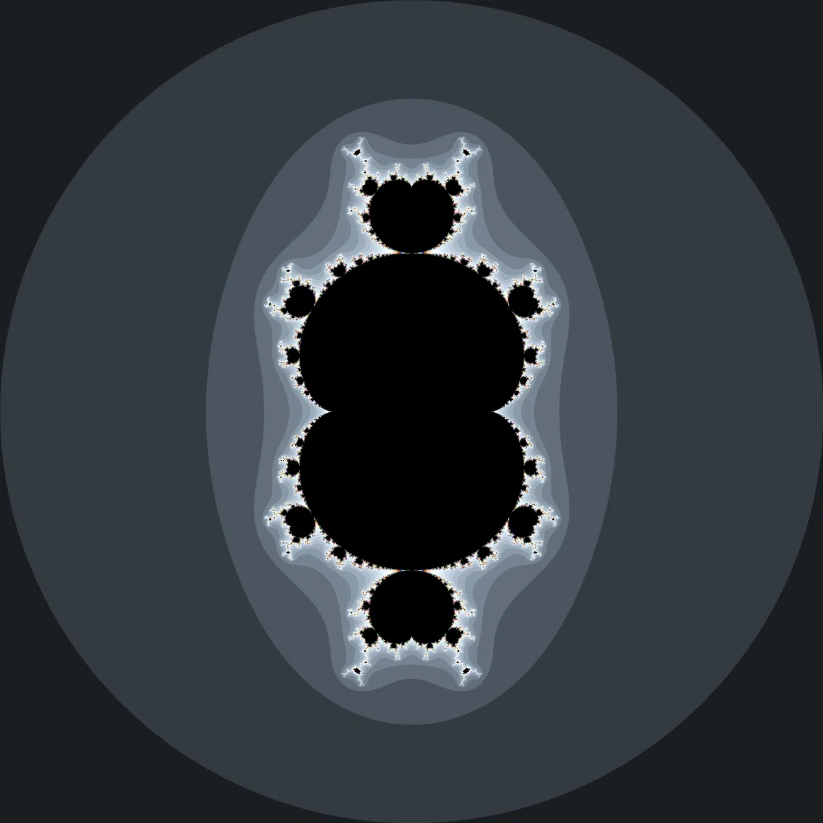
Multibrot set
void setup(){
  size(2000,2000);
  background(0);
  noStroke();
  double x,y,px,py,a,b;
  boolean o;
  for(int k=0;k<2000;k++){
    for(int m=0;m<2000;m++){
      a=(double)k/500.0-2.0;
      b=(double)m/500.0-2.0;
      x=0;
      y=0;
      o=true;
      for(int n=1;n<=500&&o;n++){
        px=x;
        py=y;
        x=px*px*px-3.0*px*py*py+a;//ここを変える
        y=3.0*px*px*py-py*py*py+b;//ここを変える
        if(x*x+y*y>4){
          o=false;
          fill(cr(n*7),cr(n*8),cr(n*9));
          rect(k,m,1,1);
        }
      }
    }
  }
}

float cr(float n){
  return (n%256)*(256-(n%256))/65;
}
A $${d}$$-order Multibrot set is the set of constants $${c}$$ for which the sequence $${z_0=0,z_{n+1}=z_n^d+c}$$ does not diverge to infinity.
If $${d=2}$$, it becomes the standard Mandelbrot set, and for $${d>3}$$, you can obtain beautiful images by zooming in, just like with the Mandelbrot set.

Burning Ship fractal

void setup(){
  size(2000,2000);
  background(0);
  noStroke();
  double x,y,px,py,a,b;
  boolean o;
  for(int k=0;k<2000;k++){
    for(int m=0;m<2000;m++){
      a=(double)k/500.0-2.0;
      b=(double)m/500.0-2.0;
      x=0.3;
      y=0.5;
      o=true;
      for(int n=1;n<=500&&o;n++){
        px=abs(x);//ここを変更
        py=abs(y);//ここを変更
        x=px*px-py*py+a;
        y=2.0*px*py+b;
        if(x*x+y*y>4){
          o=false;
          fill(cr(n*7),cr(n*8),cr(n*9));
          rect(k,m,1,1);
        }
      }
    }
  }
}

float cr(float n){
  return (n%256)*(256-(n%256))/65;
}

double abs(double x){//ここから追加
  if(x<0){
    return -x;
  }else{
    return x;
  }
}
The Burning Ship fractal is a figure generated when the sequence used for calculating the Mandelbrot set is changed to $${z_{n+1}=(|Re(z_n)|+|Im(z_n)|i)^2+c}$$ (where $${Re(z)}$$ and $${Im(z)}$$ are the real and imaginary parts of $${z}$$).
Processing has a built-in function for calculating absolute values, but it does not seem to support the double type, so I have created my own function.
The Burning Ship fractal is characterized by its ship-like shape, and if you zoom in near the center of the left edge, you can see many small ships lined up.

Note that unlike the Mandelbrot set, the Burning Ship fractal has regions where calculation acceleration does not work well ($${z_n}$$ does not converge to a periodic sequence).

Filled Julia set

void setup(){
  size(2000,2000);
  background(0);
  noStroke();
  double x,y,px,py,a,b;
  boolean o;
  for(int k=0;k<2000;k++){
    for(int m=0;m<2000;m++){
      //ここから変更
      a=0.3;
      b=0.5;
      x=(double)k/500.0-2.0;
      y=(double)m/500.0-2.0;
      //ここまで変更
      o=true;
      for(int n=1;n<=500&&o;n++){
        px=x;
        py=y;
        x=px*px-py*py+a;
        y=2.0*px*py+b;
        if(x*x+y*y>4){
          o=false;
          fill(cr(n*7),cr(n*8),cr(n*9));
          rect(k,m,1,1);
        }
      }
    }
  }
}

float cr(float n){
  return (n%256)*(256-(n%256))/65;
}
A filled Julia set of $${f(z)}$$ is the set of initial values $${z_0}$$ for which the sequence $${z_{n+1}=f(z_n)}$$ does not diverge to infinity.
By changing the values of a and b or the part corresponding to the $${z_n}$$ formula, you can generate Julia sets with different appearances.


